library(tidyverse)
library(caret)
library(car)
library(glmnet)6 Linear Regression
Coverage: Linear Regression, General Linear Regression, Lasso, Ridge, Elastic Net Regression
6.1 Theoritical Knowledge
The multivariate linear Regression \(y = X \beta\) with loss function \(Q = \left\| (y - X \beta) \right\|^2 = (y - X \beta) ^T (y - X \beta)\)
\[ \frac{\partial Q}{\partial \beta} = -2X^Ty + 2X^TX\beta = 0 \\ \to \hat{\beta} = {(X^TX)}^{-1}X^Ty \]
H is called Hat Matrix where: \(\hat{y} = X \hat{\beta} = X (X^TX)^{-1}X^Ty = Hy\)
Normal Equation: \((X^TX)\hat{\beta} = X^Ty \to X^T(y-X\hat{\beta}) = 0\)
\[ R^2 = \frac{SSR}{SST} = 1 - \frac{SSE}{SST} \]
\[ \text{Adjusted-}R^2 = \frac{SSR/k}{SST/(n-1)} = 1- \frac{SSE/(n-k-1)}{SST/(n-1)} \]
Notice that here SSE means Sum Square Error, and SSR means Sum Square Regression. Sometimes you might see ESS which is Explained Sum Square which equals to SSR here, and RSS is Residual Sum Square.
In R, use lm() to fit a linear regression model.
6.2 Example: diamonds dataset
data(diamonds)
head(diamonds)
# A tibble: 6 × 10
carat cut color clarity depth table price x y z
<dbl> <ord> <ord> <ord> <dbl> <dbl> <int> <dbl> <dbl> <dbl>
1 0.23 Ideal E SI2 61.5 55 326 3.95 3.98 2.43
2 0.21 Premium E SI1 59.8 61 326 3.89 3.84 2.31
3 0.23 Good E VS1 56.9 65 327 4.05 4.07 2.31
4 0.29 Premium I VS2 62.4 58 334 4.2 4.23 2.63
5 0.31 Good J SI2 63.3 58 335 4.34 4.35 2.75
6 0.24 Very Good J VVS2 62.8 57 336 3.94 3.96 2.48sum(is.na(diamonds))[1] 0str(diamonds)tibble [53,940 × 10] (S3: tbl_df/tbl/data.frame)
$ carat : num [1:53940] 0.23 0.21 0.23 0.29 0.31 0.24 0.24 0.26 0.22 0.23 ...
$ cut : Ord.factor w/ 5 levels "Fair"<"Good"<..: 5 4 2 4 2 3 3 3 1 3 ...
$ color : Ord.factor w/ 7 levels "D"<"E"<"F"<"G"<..: 2 2 2 6 7 7 6 5 2 5 ...
$ clarity: Ord.factor w/ 8 levels "I1"<"SI2"<"SI1"<..: 2 3 5 4 2 6 7 3 4 5 ...
$ depth : num [1:53940] 61.5 59.8 56.9 62.4 63.3 62.8 62.3 61.9 65.1 59.4 ...
$ table : num [1:53940] 55 61 65 58 58 57 57 55 61 61 ...
$ price : int [1:53940] 326 326 327 334 335 336 336 337 337 338 ...
$ x : num [1:53940] 3.95 3.89 4.05 4.2 4.34 3.94 3.95 4.07 3.87 4 ...
$ y : num [1:53940] 3.98 3.84 4.07 4.23 4.35 3.96 3.98 4.11 3.78 4.05 ...
$ z : num [1:53940] 2.43 2.31 2.31 2.63 2.75 2.48 2.47 2.53 2.49 2.39 ...6.2.1 Without preprocessing
fit1 <- lm(price~., diamonds)
summary(fit1)
Call:
lm(formula = price ~ ., data = diamonds)

Residuals:
     Min       1Q   Median       3Q      Max
-21376.0   -592.4   -183.5    376.4  10694.2

Coefficients:
             Estimate Std. Error  t value Pr(>|t|)
(Intercept)  5753.762    396.630   14.507  < 2e-16 ***
carat       11256.978     48.628  231.494  < 2e-16 ***
cut.L         584.457     22.478   26.001  < 2e-16 ***
cut.Q        -301.908     17.994  -16.778  < 2e-16 ***
cut.C         148.035     15.483    9.561  < 2e-16 ***
cut^4         -20.794     12.377   -1.680  0.09294 .
color.L     -1952.160     17.342 -112.570  < 2e-16 ***
color.Q      -672.054     15.777  -42.597  < 2e-16 ***
color.C      -165.283     14.725  -11.225  < 2e-16 ***
color^4        38.195     13.527    2.824  0.00475 **
color^5       -95.793     12.776   -7.498 6.59e-14 ***
color^6       -48.466     11.614   -4.173 3.01e-05 ***
clarity.L    4097.431     30.259  135.414  < 2e-16 ***
clarity.Q   -1925.004     28.227  -68.197  < 2e-16 ***
clarity.C     982.205     24.152   40.668  < 2e-16 ***
clarity^4    -364.918     19.285  -18.922  < 2e-16 ***
clarity^5     233.563     15.752   14.828  < 2e-16 ***
clarity^6       6.883     13.715    0.502  0.61575
clarity^7      90.640     12.103    7.489 7.06e-14 ***
depth         -63.806      4.535  -14.071  < 2e-16 ***
table         -26.474      2.912   -9.092  < 2e-16 ***
x           -1008.261     32.898  -30.648  < 2e-16 ***
y               9.609     19.333    0.497  0.61918
z             -50.119     33.486   -1.497  0.13448
---
Signif. codes:  0 '***' 0.001 '**' 0.01 '*' 0.05 '.' 0.1 ' ' 1

Residual standard error: 1130 on 53916 degrees of freedom
Multiple R-squared:  0.9198,    Adjusted R-squared:  0.9198
F-statistic: 2.688e+04 on 23 and 53916 DF, p-value: < 2.2e-16par(mfrow = c(2, 2))
plot(fit1)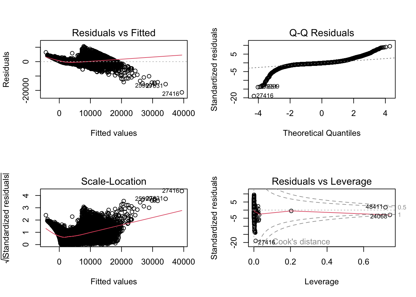
Variance Inflation Factor (VIF) is useful to detect multicollinear.
vif(fit1) GVIF Df GVIF^(1/(2*Df))
carat 22.439582 1 4.737044
cut 1.945645 4 1.086758
color 1.178326 6 1.013768
clarity 1.347474 7 1.021531
depth 1.782401 1 1.335066
table 1.787765 1 1.337073
x 57.518327 1 7.584084
y 20.592160 1 4.537859
z 23.585582 1 4.856499fit1a <- lm(price~.-x-z-y, diamonds)
vif(fit1a) GVIF Df GVIF^(1/(2*Df))
carat 1.323098 1 1.150260
cut 1.926004 4 1.085381
color 1.169317 6 1.013120
clarity 1.303877 7 1.019134
depth 1.378257 1 1.173992
table 1.786714 1 1.336680summary(fit1a)
Call:
lm(formula = price ~ . - x - z - y, data = diamonds)

Residuals:
     Min       1Q   Median       3Q      Max
-16828.8   -678.7   -199.4    464.6  10341.2

Coefficients:
             Estimate Std. Error  t value Pr(>|t|)
(Intercept)  -969.661    360.432   -2.690  0.00714 **
carat        8895.194     12.079  736.390  < 2e-16 ***
cut.L         615.613     22.985   26.784  < 2e-16 ***
cut.Q        -326.638     18.390  -17.762  < 2e-16 ***
cut.C         156.333     15.814    9.886  < 2e-16 ***
cut^4         -15.975     12.648   -1.263  0.20657
color.L     -1908.010     17.718 -107.689  < 2e-16 ***
color.Q      -626.087     16.112  -38.858  < 2e-16 ***
color.C      -172.056     15.063  -11.423  < 2e-16 ***
color^4        20.319     13.833    1.469  0.14187
color^5       -85.245     13.068   -6.523 6.95e-11 ***
color^6       -50.085     11.881   -4.216 2.50e-05 ***
clarity.L    4206.854     30.867  136.290  < 2e-16 ***
clarity.Q   -1831.804     28.811  -63.580  < 2e-16 ***
clarity.C     919.725     24.672   37.278  < 2e-16 ***
clarity^4    -361.609     19.728  -18.330  < 2e-16 ***
clarity^5     213.910     16.108   13.280  < 2e-16 ***
clarity^6       2.986     14.030    0.213  0.83148
clarity^7     110.147     12.375    8.901  < 2e-16 ***
depth         -21.024      4.079   -5.154 2.56e-07 ***
table         -24.803      2.978   -8.329  < 2e-16 ***
---
Signif. codes:  0 '***' 0.001 '**' 0.01 '*' 0.05 '.' 0.1 ' ' 1

Residual standard error: 1156 on 53919 degrees of freedom
Multiple R-squared:  0.9161,    Adjusted R-squared:  0.916
F-statistic: 2.942e+04 on 20 and 53919 DF, p-value: < 2.2e-16par(mfrow = c(2, 2))
plot(fit1a)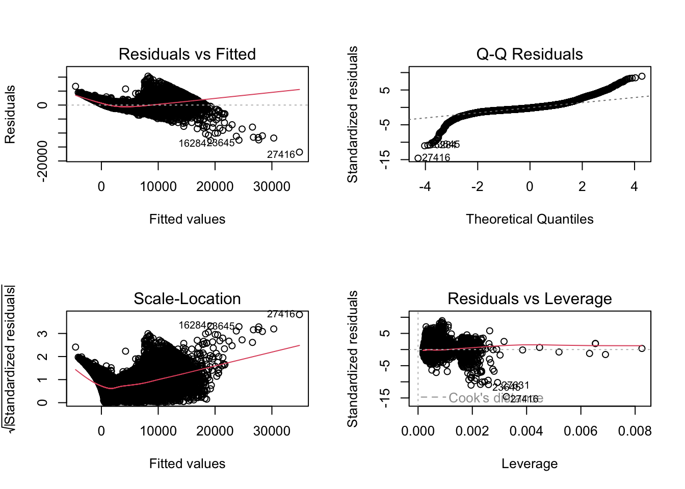
fit2 <- lm(log(price)~., diamonds)
summary(fit2)
Call:
lm(formula = log(price) ~ ., data = diamonds)

Residuals:
    Min      1Q  Median      3Q     Max
-2.2544 -0.0911  0.0015  0.0902 10.2241

Coefficients:
              Estimate Std. Error  t value Pr(>|t|)
(Intercept) -2.5530834  0.0616229  -41.431  < 2e-16 ***
carat       -0.6120540  0.0075551  -81.012  < 2e-16 ***
cut.L        0.1045411  0.0034923   29.934  < 2e-16 ***
cut.Q       -0.0370562  0.0027956  -13.255  < 2e-16 ***
cut.C        0.0371749  0.0024056   15.454  < 2e-16 ***
cut^4        0.0115784  0.0019229    6.021 1.74e-09 ***
color.L     -0.4526278  0.0026943 -167.993  < 2e-16 ***
color.Q     -0.1035542  0.0024512  -42.246  < 2e-16 ***
color.C     -0.0118522  0.0022878   -5.181 2.22e-07 ***
color^4      0.0188754  0.0021016    8.982  < 2e-16 ***
color^5     -0.0068063  0.0019850   -3.429 0.000606 ***
color^6      0.0021343  0.0018044    1.183 0.236892
clarity.L    0.8907095  0.0047012  189.466  < 2e-16 ***
clarity.Q   -0.2599052  0.0043856  -59.264  < 2e-16 ***
clarity.C    0.1435463  0.0037523   38.255  < 2e-16 ***
clarity^4   -0.0662975  0.0029962  -22.127  < 2e-16 ***
clarity^5    0.0285591  0.0024473   11.670  < 2e-16 ***
clarity^6   -0.0039048  0.0021309   -1.833 0.066881 .
clarity^7    0.0290474  0.0018805   15.447  < 2e-16 ***
depth        0.0521543  0.0007045   74.028  < 2e-16 ***
table        0.0089978  0.0004524   19.890  < 2e-16 ***
x            1.1646945  0.0051112  227.871  < 2e-16 ***
y            0.0325386  0.0030037   10.833  < 2e-16 ***
z            0.0427049  0.0052026    8.208 2.29e-16 ***
---
Signif. codes:  0 '***' 0.001 '**' 0.01 '*' 0.05 '.' 0.1 ' ' 1

Residual standard error: 0.1756 on 53916 degrees of freedom
Multiple R-squared:  0.9701,    Adjusted R-squared:  0.9701
F-statistic: 7.597e+04 on 23 and 53916 DF, p-value: < 2.2e-16par(mfrow = c(2, 2))
plot(fit2)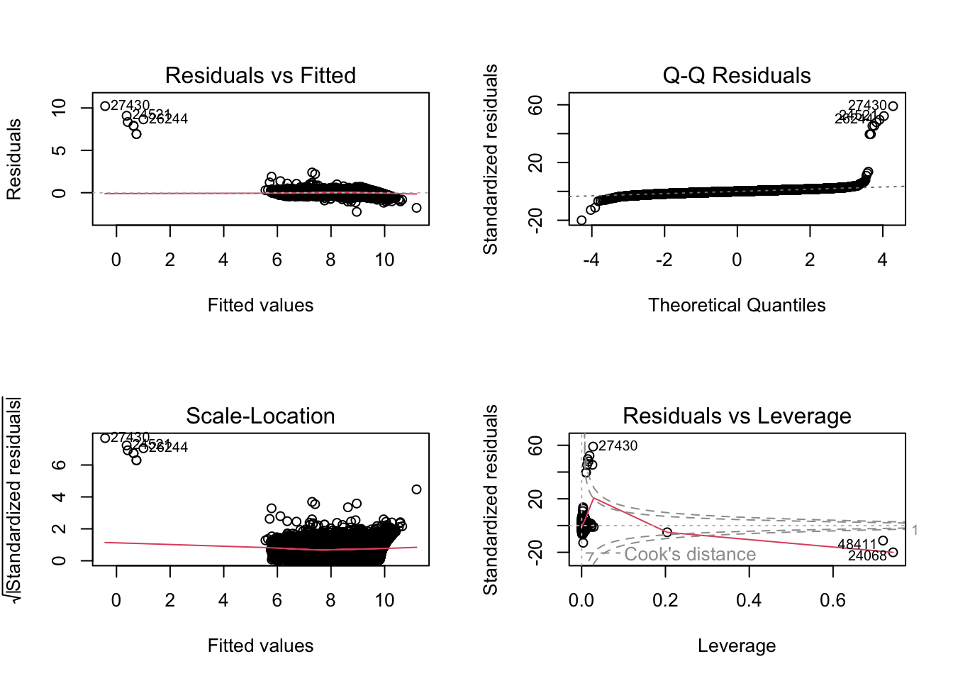
vif(fit2) GVIF Df GVIF^(1/(2*Df))
carat 22.439582 1 4.737044
cut 1.945645 4 1.086758
color 1.178326 6 1.013768
clarity 1.347474 7 1.021531
depth 1.782401 1 1.335066
table 1.787765 1 1.337073
x 57.518327 1 7.584084
y 20.592160 1 4.537859
z 23.585582 1 4.856499fit2a <- lm(log(price)~.-x-z-y, diamonds)
vif(fit2a) GVIF Df GVIF^(1/(2*Df))
carat 1.323098 1 1.150260
cut 1.926004 4 1.085381
color 1.169317 6 1.013120
clarity 1.303877 7 1.019134
depth 1.378257 1 1.173992
table 1.786714 1 1.336680summary(fit2a)
Call:
lm(formula = log(price) ~ . - x - z - y, data = diamonds)

Residuals:
    Min      1Q  Median      3Q     Max
-5.9717 -0.2181  0.0572  0.2479  1.6083

Coefficients:
              Estimate Std. Error t value Pr(>|t|)
(Intercept)  5.5193818  0.1055868  52.273  < 2e-16 ***
carat        2.1946870  0.0035386 620.211  < 2e-16 ***
cut.L        0.0682284  0.0067332  10.133  < 2e-16 ***
cut.Q       -0.0090647  0.0053872  -1.683   0.0925 .
cut.C        0.0291522  0.0046325   6.293 3.14e-10 ***
cut^4        0.0065684  0.0037051   1.773   0.0763 .
color.L     -0.5051100  0.0051903 -97.318  < 2e-16 ***
color.Q     -0.1582296  0.0047199 -33.524  < 2e-16 ***
color.C     -0.0038111  0.0044125  -0.864   0.3877
color^4      0.0400952  0.0040522   9.895  < 2e-16 ***
color^5     -0.0192706  0.0038283  -5.034 4.82e-07 ***
color^6      0.0041225  0.0034805   1.184   0.2362
clarity.L    0.7615612  0.0090423  84.222  < 2e-16 ***
clarity.Q   -0.3710533  0.0084401 -43.963  < 2e-16 ***
clarity.C    0.2181958  0.0072276  30.189  < 2e-16 ***
clarity^4   -0.0704719  0.0057792 -12.194  < 2e-16 ***
clarity^5    0.0521882  0.0047187  11.060  < 2e-16 ***
clarity^6    0.0006772  0.0041100   0.165   0.8691
clarity^7    0.0058294  0.0036253   1.608   0.1078
depth        0.0000854  0.0011950   0.071   0.9430
table        0.0068963  0.0008723   7.906 2.71e-15 ***
---
Signif. codes:  0 '***' 0.001 '**' 0.01 '*' 0.05 '.' 0.1 ' ' 1

Residual standard error: 0.3387 on 53919 degrees of freedom
Multiple R-squared:  0.8886,    Adjusted R-squared:  0.8886
F-statistic: 2.151e+04 on 20 and 53919 DF, p-value: < 2.2e-16par(mfrow = c(2, 2))
plot(fit2a)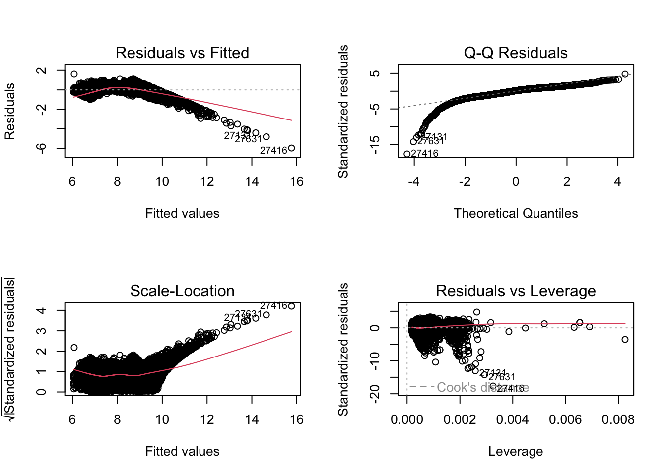
The second model looks better.
6.2.2 With preprocessing
new_diamonds <- diamonds %>%
    predict(dummyVars(price ~ ., data = ., sep = "_", levelsOnly = FALSE), newdata = .) %>%
    as.data.frame() %>%
    mutate(logprice = log(diamonds$price))
colnames(new_diamonds) <- gsub("\\^", "_", colnames(new_diamonds))

set.seed(42)
training.idx <- new_diamonds$logprice %>%
    createDataPartition(p = 0.75, list = F)
trainset <- new_diamonds[training.idx, ]
testset <- new_diamonds[-training.idx, ]

prepproc <- preProcess(trainset, method = c("center", "scale"))
trainset.scaled <- predict(prepproc, trainset)
testset.scaled <- predict(prepproc, testset)

mu <- prepproc$mean["logprice"]
sigma <- prepproc$std["logprice"]

train.x <- trainset.scaled %>% select(-logprice)
test.x <- testset.scaled %>% select(-logprice)
fit3 <- lm(logprice~.-x-z-y, trainset.scaled)
summary(fit3)
Call:
lm(formula = logprice ~ . - x - z - y, data = trainset.scaled)

Residuals:
    Min      1Q  Median      3Q     Max
-4.7768 -0.2137  0.0560  0.2444  1.5795

Coefficients:
              Estimate Std. Error t value Pr(>|t|)
(Intercept) -3.959e-14  1.653e-03   0.000   1.0000
carat        1.025e+00  1.899e-03 540.026  < 2e-16 ***
cut.L        2.457e-02  2.677e-03   9.179  < 2e-16 ***
cut.Q       -4.757e-03  2.791e-03  -1.705   0.0883 .
cut.C        1.268e-02  2.237e-03   5.667 1.46e-08 ***
cut_4        2.137e-03  1.869e-03   1.143   0.2530
color.L     -1.603e-01  1.888e-03 -84.918  < 2e-16 ***
color.Q     -5.285e-02  1.831e-03 -28.871  < 2e-16 ***
color.C      2.460e-05  1.810e-03   0.014   0.9892
color_4      1.505e-02  1.782e-03   8.448  < 2e-16 ***
color_5     -6.681e-03  1.702e-03  -3.926 8.65e-05 ***
color_6      5.532e-04  1.681e-03   0.329   0.7420
clarity.L    1.891e-01  2.585e-03  73.170  < 2e-16 ***
clarity.Q   -8.582e-02  2.271e-03 -37.790  < 2e-16 ***
clarity.C    6.390e-02  2.479e-03  25.779  < 2e-16 ***
clarity_4   -2.354e-02  2.295e-03 -10.257  < 2e-16 ***
clarity_5    1.698e-02  2.012e-03   8.440  < 2e-16 ***
clarity_6   -1.291e-03  1.878e-03  -0.687   0.4920
clarity_7    1.763e-03  1.755e-03   1.005   0.3151
depth       -3.771e-05  1.929e-03  -0.020   0.9844
table        1.549e-02  2.215e-03   6.990 2.80e-12 ***
---
Signif. codes:  0 '***' 0.001 '**' 0.01 '*' 0.05 '.' 0.1 ' ' 1

Residual standard error: 0.3325 on 40436 degrees of freedom
Multiple R-squared:  0.8895,    Adjusted R-squared:  0.8895
F-statistic: 1.628e+04 on 20 and 40436 DF, p-value: < 2.2e-16vif(fit3) carat cut.L cut.Q cut.C cut_4 color.L color.Q color.C
1.319348 2.621717 2.850233 1.832031 1.278920 1.304379 1.226508 1.199441
color_4 color_5 color_6 clarity.L clarity.Q clarity.C clarity_4 clarity_5
1.161859 1.059918 1.033804 2.445376 1.887271 2.248751 1.926817 1.481558
clarity_6 clarity_7 depth table
1.291236 1.126544 1.362239 1.796295 par(mfrow = c(2, 2))
plot(fit3)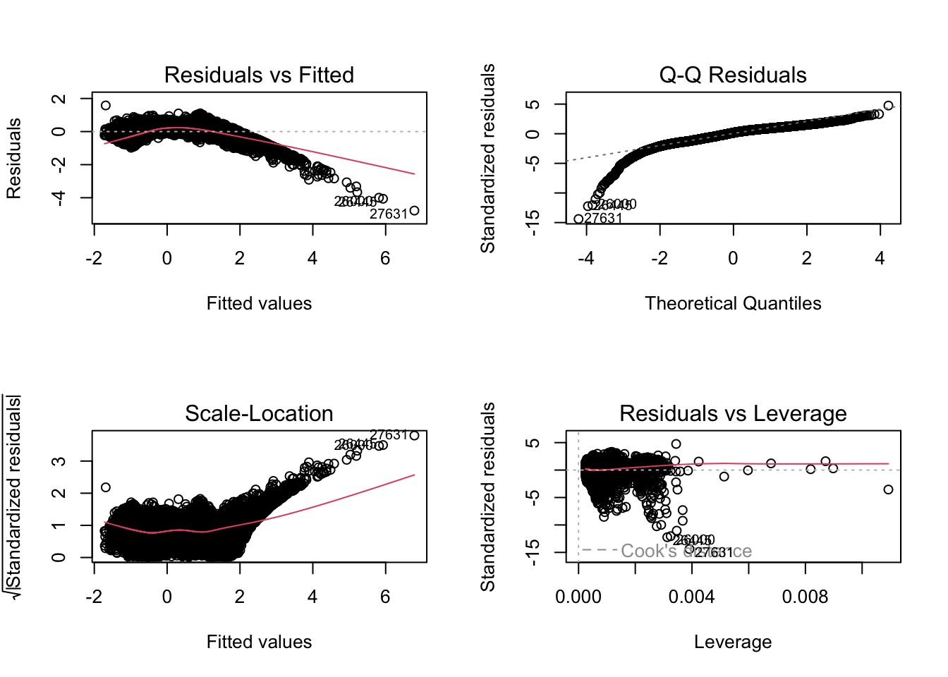
ytr.true <- exp(trainset$logprice)
yte.true <- exp(testset$logprice)
ytr.pred3 <- exp(predict(fit3, train.x) * sigma + mu)
yte.pred3 <- exp(predict(fit3, test.x) * sigma + mu)


pf.lm <- data.frame(
    model = "lm",
    train.mse = mean((ytr.pred3-ytr.true)^2),
    test.mse = mean((yte.pred3-yte.true)^2)
)
pf.lm
model train.mse test.mse
1 lm 229599179 4206268380pf.linearRegression <- postResample(
pred = yte.pred3,
obs = yte.true
)6.3 Stepwise regression and best subset
There’re two Information Criterions:
Akaike Information Criterion \(\text{AIC} = - 2 \log{L} + 2 k\)
Bayesian Information Criterion (aka Schwarz IC) \(\text{BIC} = - 2 \log{L} + k \log{N}\)
Here \(L\) denotes the maximum likelihood, \(k\) denotes number of parameters in the model, and \(N\) denotes the number of observations.
When sample size \(N > 7 (e^2 \approx 7.389056)\), BIC is more likely to drop variables compare with AIC.
\[\text{Criterion}=\text{Penalty for Error}+\text{Penalty for Complexity}\]
The smaller, the better.
Stepwise Regression: Backward (start from full model) or Forward (start from null model) then drop or add variables based on greedy strategy.
Best Subset Regression: Iterate all subsets of full variables, then find the best subset.
6.3.1 Stepwise Regression
library(MASS)
Attaching package: 'MASS'The following object is masked from 'package:dplyr':
select6.3.1.1 Backward (start from full model)
set k = 2 for AIC, k = log(nrow(train.data)) for BIC.
When you set trace = 1, every step will be printed.
fit_s1a <- lm(logprice~., trainset.scaled)
fit_step_backward <- stepAIC(fit_s1a, k = log(nrow(trainset.scaled)), trace = 0) # MASS pkg
summary(fit_step_backward)
Call:
lm(formula = logprice ~ carat + cut.L + cut.Q + cut.C + cut_4 +
    color.L + color.Q + color.C + color_4 + clarity.L + clarity.Q +
    clarity.C + clarity_4 + clarity_5 + clarity_7 + depth + table +
    x + y + z, data = trainset.scaled)

Residuals:
    Min      1Q  Median      3Q     Max
-2.2146 -0.0910  0.0021  0.0900  9.8143

Coefficients:
              Estimate Std. Error  t value Pr(>|t|)
(Intercept) -1.795e-14  8.879e-04    0.000  1.00000
carat       -2.533e-01  4.176e-03  -60.651  < 2e-16 ***
cut.L        3.546e-02  1.438e-03   24.663  < 2e-16 ***
cut.Q       -1.589e-02  1.500e-03  -10.593  < 2e-16 ***
cut.C        1.484e-02  1.203e-03   12.338  < 2e-16 ***
cut_4        5.114e-03  1.005e-03    5.090 3.60e-07 ***
color.L     -1.442e-01  1.015e-03 -142.104  < 2e-16 ***
color.Q     -3.530e-02  9.829e-04  -35.917  < 2e-16 ***
color.C     -3.310e-03  9.605e-04   -3.446  0.00057 ***
color_4      8.162e-03  9.336e-04    8.743  < 2e-16 ***
clarity.L    2.220e-01  1.386e-03  160.173  < 2e-16 ***
clarity.Q   -6.169e-02  1.210e-03  -50.991  < 2e-16 ***
clarity.C    4.353e-02  1.322e-03   32.916  < 2e-16 ***
clarity_4   -2.260e-02  1.190e-03  -18.988  < 2e-16 ***
clarity_5    1.105e-02  1.053e-03   10.498  < 2e-16 ***
clarity_7    1.260e-02  9.034e-04   13.949  < 2e-16 ***
depth        7.160e-02  1.159e-03   61.777  < 2e-16 ***
table        2.002e-02  1.190e-03   16.821  < 2e-16 ***
x            1.276e+00  6.303e-03  202.424  < 2e-16 ***
y            1.456e-02  3.555e-03    4.096 4.21e-05 ***
z            2.997e-02  3.932e-03    7.622 2.55e-14 ***
---
Signif. codes:  0 '***' 0.001 '**' 0.01 '*' 0.05 '.' 0.1 ' ' 1

Residual standard error: 0.1786 on 40436 degrees of freedom
Multiple R-squared:  0.9681,    Adjusted R-squared:  0.9681
F-statistic: 6.14e+04 on 20 and 40436 DF,  p-value: < 2.2e-16
ytr.pred.sb <- exp(fit_step_backward %>% predict(train.x) * sigma + mu)
yte.pred.sb <- exp(fit_step_backward %>% predict(test.x) * sigma + mu)
pf.lm.sb <- data.frame(
model = "Stepwise-Backward",
train.mse = mean((ytr.pred.sb-ytr.true)^2),
test.mse = mean((yte.pred.sb-yte.true)^2)
)
pf.lm.sb model train.mse test.mse
1 Stepwise-Backward 1200659 1243213pf.Stepwise.Backward <- postResample(
pred = yte.pred.sb,
obs = yte.true
)6.3.1.2 Forward (start from null model)
fit_s2a <- lm(logprice~1, trainset.scaled)
fit_s2b <- lm(logprice~., trainset.scaled)
fit_step_forward <- stepAIC(fit_s2a, scope = list(lower = fit_s2a, upper = fit_s2b),
                        direction = "forward", k = log(nrow(trainset.scaled)), trace = 0) # MASS pkg
summary(fit_step_forward)
Call:
lm(formula = logprice ~ x + clarity.L + color.L + carat + depth +
    clarity.Q + color.Q + clarity.C + clarity_4 + cut.L + table +
    clarity_7 + cut_4 + clarity_5 + color_4 + z + cut.C + cut.Q +
    y + color.C, data = trainset.scaled)

Residuals:
    Min      1Q  Median      3Q     Max
-2.2146 -0.0910  0.0021  0.0900  9.8143

Coefficients:
              Estimate Std. Error  t value Pr(>|t|)
(Intercept) -1.795e-14  8.879e-04    0.000  1.00000
x            1.276e+00  6.303e-03  202.424  < 2e-16 ***
clarity.L    2.220e-01  1.386e-03  160.173  < 2e-16 ***
color.L     -1.442e-01  1.015e-03 -142.104  < 2e-16 ***
carat       -2.533e-01  4.176e-03  -60.651  < 2e-16 ***
depth        7.160e-02  1.159e-03   61.777  < 2e-16 ***
clarity.Q   -6.169e-02  1.210e-03  -50.991  < 2e-16 ***
color.Q     -3.530e-02  9.829e-04  -35.917  < 2e-16 ***
clarity.C    4.353e-02  1.322e-03   32.916  < 2e-16 ***
clarity_4   -2.260e-02  1.190e-03  -18.988  < 2e-16 ***
cut.L        3.546e-02  1.438e-03   24.663  < 2e-16 ***
table        2.002e-02  1.190e-03   16.821  < 2e-16 ***
clarity_7    1.260e-02  9.034e-04   13.949  < 2e-16 ***
cut_4        5.114e-03  1.005e-03    5.090 3.60e-07 ***
clarity_5    1.105e-02  1.053e-03   10.498  < 2e-16 ***
color_4      8.162e-03  9.336e-04    8.743  < 2e-16 ***
z            2.997e-02  3.932e-03    7.622 2.55e-14 ***
cut.C        1.484e-02  1.203e-03   12.338  < 2e-16 ***
cut.Q       -1.589e-02  1.500e-03  -10.593  < 2e-16 ***
y            1.456e-02  3.555e-03    4.096 4.21e-05 ***
color.C     -3.310e-03  9.605e-04   -3.446  0.00057 ***
---
Signif. codes:  0 '***' 0.001 '**' 0.01 '*' 0.05 '.' 0.1 ' ' 1

Residual standard error: 0.1786 on 40436 degrees of freedom
Multiple R-squared:  0.9681,    Adjusted R-squared:  0.9681
F-statistic: 6.14e+04 on 20 and 40436 DF,  p-value: < 2.2e-16
ytr.pred.sf <- exp(fit_step_forward %>% predict(train.x) * sigma + mu)
yte.pred.sf <- exp(fit_step_forward %>% predict(test.x) * sigma + mu)
pf.lm.sf <- data.frame(
model = "Stepwise-Forward",
train.mse = mean((ytr.pred.sf-ytr.true)^2),
test.mse = mean((yte.pred.sf-yte.true)^2)
)
pf.lm.sb model train.mse test.mse
1 Stepwise-Backward 1200659 1243213pf.Stepwise.Forward <- postResample(
pred = yte.pred.sf,
obs = yte.true
)6.3.2 Best Subset Regression
library(leaps)fit_bs <- regsubsets(logprice~., trainset.scaled, nvmax = 30)
# nvmax = 30: sets the maximum number of predictors to consider.
summary(fit_bs)Subset selection object
Call: regsubsets.formula(logprice ~ ., trainset.scaled, nvmax = 30)
23 Variables (and intercept)
Forced in Forced out
carat FALSE FALSE
cut.L FALSE FALSE
cut.Q FALSE FALSE
cut.C FALSE FALSE
cut_4 FALSE FALSE
color.L FALSE FALSE
color.Q FALSE FALSE
color.C FALSE FALSE
color_4 FALSE FALSE
color_5 FALSE FALSE
color_6 FALSE FALSE
clarity.L FALSE FALSE
clarity.Q FALSE FALSE
clarity.C FALSE FALSE
clarity_4 FALSE FALSE
clarity_5 FALSE FALSE
clarity_6 FALSE FALSE
clarity_7 FALSE FALSE
depth FALSE FALSE
table FALSE FALSE
x FALSE FALSE
y FALSE FALSE
z FALSE FALSE
1 subsets of each size up to 23
Selection Algorithm: exhaustive
carat cut.L cut.Q cut.C cut_4 color.L color.Q color.C color_4 color_5
1 ( 1 ) " " " " " " " " " " " " " " " " " " " "
2 ( 1 ) " " " " " " " " " " " " " " " " " " " "
3 ( 1 ) " " " " " " " " " " "*" " " " " " " " "
4 ( 1 ) "*" " " " " " " " " "*" " " " " " " " "
5 ( 1 ) "*" " " " " " " " " "*" " " " " " " " "
6 ( 1 ) "*" " " " " " " " " "*" " " " " " " " "
7 ( 1 ) "*" " " " " " " " " "*" "*" " " " " " "
8 ( 1 ) "*" " " " " " " " " "*" "*" " " " " " "
9 ( 1 ) "*" " " " " " " " " "*" "*" " " " " " "
10 ( 1 ) "*" "*" " " " " " " "*" "*" " " " " " "
11 ( 1 ) "*" "*" " " " " " " "*" "*" " " " " " "
12 ( 1 ) "*" "*" " " " " " " "*" "*" " " " " " "
13 ( 1 ) "*" "*" " " " " "*" "*" "*" " " " " " "
14 ( 1 ) "*" "*" "*" "*" " " "*" "*" " " " " " "
15 ( 1 ) "*" "*" "*" "*" " " "*" "*" " " " " " "
16 ( 1 ) "*" "*" "*" "*" " " "*" "*" " " "*" " "
17 ( 1 ) "*" "*" "*" "*" " " "*" "*" " " "*" " "
18 ( 1 ) "*" "*" "*" "*" "*" "*" "*" " " "*" " "
19 ( 1 ) "*" "*" "*" "*" "*" "*" "*" " " "*" " "
20 ( 1 ) "*" "*" "*" "*" "*" "*" "*" "*" "*" " "
21 ( 1 ) "*" "*" "*" "*" "*" "*" "*" "*" "*" " "
22 ( 1 ) "*" "*" "*" "*" "*" "*" "*" "*" "*" "*"
23 ( 1 ) "*" "*" "*" "*" "*" "*" "*" "*" "*" "*"
color_6 clarity.L clarity.Q clarity.C clarity_4 clarity_5 clarity_6
1 ( 1 ) " " " " " " " " " " " " " "
2 ( 1 ) " " "*" " " " " " " " " " "
3 ( 1 ) " " "*" " " " " " " " " " "
4 ( 1 ) " " "*" " " " " " " " " " "
5 ( 1 ) " " "*" " " " " " " " " " "
6 ( 1 ) " " "*" "*" " " " " " " " "
7 ( 1 ) " " "*" "*" " " " " " " " "
8 ( 1 ) " " "*" "*" "*" " " " " " "
9 ( 1 ) " " "*" "*" "*" "*" " " " "
10 ( 1 ) " " "*" "*" "*" "*" " " " "
11 ( 1 ) " " "*" "*" "*" "*" " " " "
12 ( 1 ) " " "*" "*" "*" "*" " " " "
13 ( 1 ) " " "*" "*" "*" "*" " " " "
14 ( 1 ) " " "*" "*" "*" "*" " " " "
15 ( 1 ) " " "*" "*" "*" "*" "*" " "
16 ( 1 ) " " "*" "*" "*" "*" "*" " "
17 ( 1 ) " " "*" "*" "*" "*" "*" " "
18 ( 1 ) " " "*" "*" "*" "*" "*" " "
19 ( 1 ) " " "*" "*" "*" "*" "*" " "
20 ( 1 ) " " "*" "*" "*" "*" "*" " "
21 ( 1 ) " " "*" "*" "*" "*" "*" "*"
22 ( 1 ) " " "*" "*" "*" "*" "*" "*"
23 ( 1 ) "*" "*" "*" "*" "*" "*" "*"
clarity_7 depth table x y z
1 ( 1 ) " " " " " " "*" " " " "
2 ( 1 ) " " " " " " "*" " " " "
3 ( 1 ) " " " " " " "*" " " " "
4 ( 1 ) " " " " " " "*" " " " "
5 ( 1 ) " " "*" " " "*" " " " "
6 ( 1 ) " " "*" " " "*" " " " "
7 ( 1 ) " " "*" " " "*" " " " "
8 ( 1 ) " " "*" " " "*" " " " "
9 ( 1 ) " " "*" " " "*" " " " "
10 ( 1 ) " " "*" " " "*" " " " "
11 ( 1 ) " " "*" "*" "*" " " " "
12 ( 1 ) "*" "*" "*" "*" " " " "
13 ( 1 ) "*" "*" "*" "*" " " " "
14 ( 1 ) "*" "*" "*" "*" " " " "
15 ( 1 ) "*" "*" "*" "*" " " " "
16 ( 1 ) "*" "*" "*" "*" " " " "
17 ( 1 ) "*" "*" "*" "*" " " "*"
18 ( 1 ) "*" "*" "*" "*" " " "*"
19 ( 1 ) "*" "*" "*" "*" "*" "*"
20 ( 1 ) "*" "*" "*" "*" "*" "*"
21 ( 1 ) "*" "*" "*" "*" "*" "*"
22 ( 1 ) "*" "*" "*" "*" "*" "*"
23 ( 1 ) "*" "*" "*" "*" "*" "*"result <- summary(fit_bs)
result$which[which.min(result$bic),](Intercept) carat cut.L cut.Q cut.C cut_4
TRUE TRUE TRUE TRUE TRUE TRUE
color.L color.Q color.C color_4 color_5 color_6
TRUE TRUE TRUE TRUE FALSE FALSE
clarity.L clarity.Q clarity.C clarity_4 clarity_5 clarity_6
TRUE TRUE TRUE TRUE TRUE FALSE
clarity_7 depth table x y z
TRUE TRUE TRUE TRUE TRUE TRUE n <- nrow(trainset.scaled) # Sample size
p <- 1:(length(result$rss)) # Model sizes (number of predictors + intercept)
aic_values <- n * log(result$rss / n) + 2 * p # Compute AIC for each model
which.min(aic_values) # Get the model size with the lowest AIC[1] 22result$which[12,](Intercept) carat cut.L cut.Q cut.C cut_4
TRUE TRUE TRUE FALSE FALSE FALSE
color.L color.Q color.C color_4 color_5 color_6
TRUE TRUE FALSE FALSE FALSE FALSE
clarity.L clarity.Q clarity.C clarity_4 clarity_5 clarity_6
TRUE TRUE TRUE TRUE FALSE FALSE
clarity_7 depth table x y z
TRUE TRUE TRUE TRUE FALSE FALSE which.max(result$adjr2)[1] 23result$which[1,](Intercept) carat cut.L cut.Q cut.C cut_4
TRUE FALSE FALSE FALSE FALSE FALSE
color.L color.Q color.C color_4 color_5 color_6
FALSE FALSE FALSE FALSE FALSE FALSE
clarity.L clarity.Q clarity.C clarity_4 clarity_5 clarity_6
FALSE FALSE FALSE FALSE FALSE FALSE
clarity_7 depth table x y z
FALSE FALSE FALSE TRUE FALSE FALSE 6.4 Lasso, Ridge and Elastic Net Regression
A general idea of penealized regression (i.e., Lasso, Ridge and Elastic Net Regression) is to add some restriction to minimize.
6.4.1 Lasso
The defination of Lasso is based on the loss function: \(Q = \left\| (y - X \beta) \right\|^2\) minimized subject to \(\left| \beta \right|_1 < t\)
It can also be written:
\[\min_{\beta \in \mathbb{R}^p} {(\frac{1}{N} \left\| (y - X \beta) \right\|^2 + \lambda \left| \beta \right|_1)}\]
Lasso will let coeffections of the model to 0, which is useful for feature selection.
set alpha = 1 for function glmnet.
lambda <- 10^seq(1,-2,length = 100)

fit.lasso <- glmnet(train.x, trainset.scaled$logprice, alpha = 1, lambda = lambda)

plot(fit.lasso, xvar = "lambda", label = TRUE)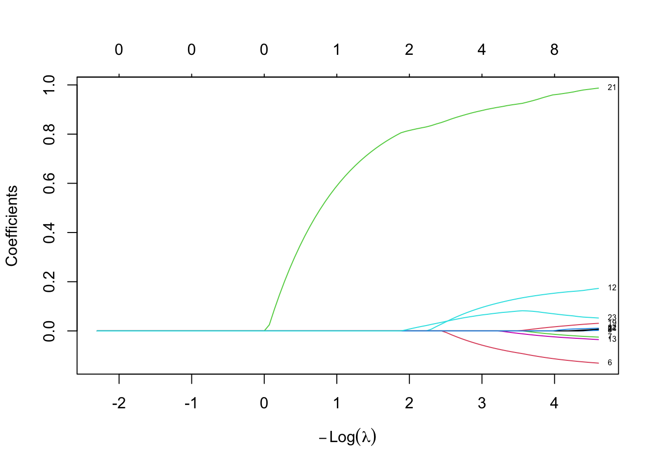
cv.lasso <- cv.glmnet(as.matrix(train.x), trainset.scaled$logprice,alpha = 1, lambda = lambda, nfolds = 10)

plot(cv.lasso)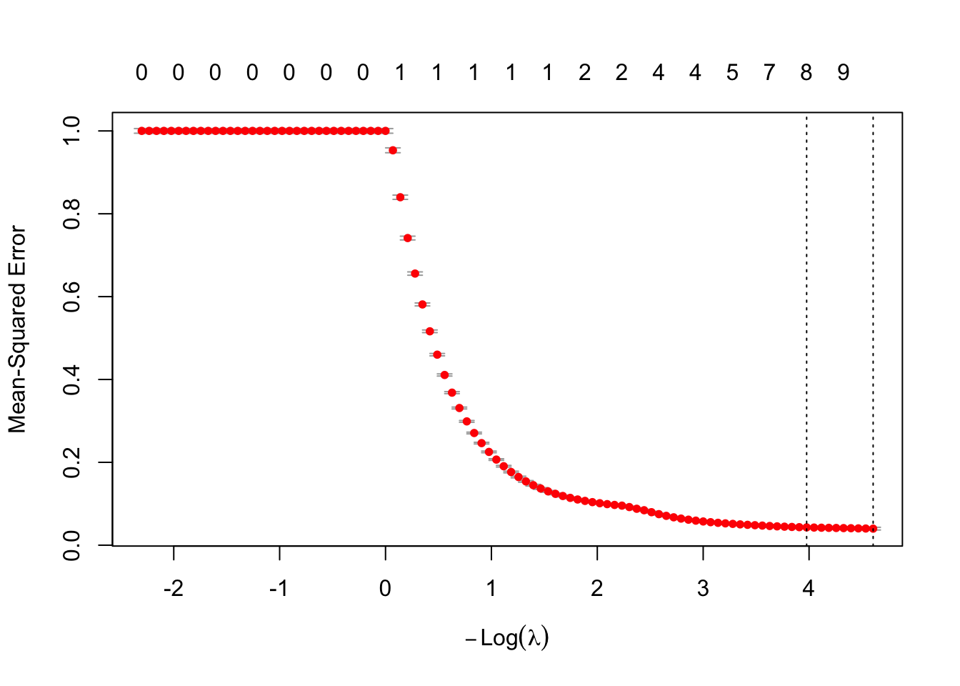
cv.lasso
Call:  cv.glmnet(x = as.matrix(train.x), y = trainset.scaled$logprice,      lambda = lambda, nfolds = 10, alpha = 1)

Measure: Mean-Squared Error

     Lambda Index Measure       SE Nonzero
min 0.01000   100 0.03992 0.003268      11
1se 0.01874    91 0.04297 0.003157       8
best_lam <- cv.lasso$lambda.min
lasso_coef <- predict(cv.lasso, s = best_lam, type = "coefficients")
import_coefs <- as.matrix(lasso_coef)
active_vars <- data.frame(
Variable = rownames(import_coefs),
Coefficient = as.numeric(import_coefs)
) %>% filter(Coefficient != 0 & Variable != "(Intercept)")
active_vars Variable Coefficient
1 cut.L 0.006033271
2 color.L -0.130907441
3 color.Q -0.025134709
4 color_4 0.002078327
5 clarity.L 0.172731638
6 clarity.Q -0.035257206
7 clarity.C 0.007961533
8 depth 0.030957031
9 x 0.987147413
10 y 0.010949118
11 z 0.052448464cat("Dropped Variables: ", rownames(import_coefs)[import_coefs[,1] == 0])Dropped Variables: carat cut.Q cut.C cut_4 color.C color_5 color_6 clarity_4 clarity_5 clarity_6 clarity_7 tableytr.pred.lasso <- exp(predict(cv.lasso,s =best_lam, newx=as.matrix(train.x)) * sigma + mu)
yte.pred.lasso <- exp(predict(cv.lasso,s = best_lam,newx= as.matrix(test.x)) * sigma + mu)
pf.lasso <- data.frame(
model = "lasso",
train.mse = mean((ytr.pred.lasso-ytr.true)^2),
test.mse = mean((yte.pred.lasso-yte.true)^2)
)
pf.lasso model train.mse test.mse
1 lasso 3193370 4703154pf.lasso2 <- postResample(
pred = yte.pred.lasso,
obs = yte.true
)6.4.2 Ridge
loss function \(Q = (y - X \beta) ^T (y - X \beta) + \beta^T \beta\)
Ridge works best in situation that OLS has high variance.
\[ \frac{\partial Q}{\partial \beta} = -2X^Ty + 2X^TX\beta + 2 \lambda \beta= 0 \\ \to \hat{\beta} = {(X^TX + \lambda I)}^{-1}X^Ty \]
set alpha = 0 for function glmnet.
lambda <- 10^seq(1,-2,length = 100)

fit.ridge <- glmnet(train.x, trainset.scaled$logprice, alpha = 0, lambda = lambda)

plot(fit.ridge, xvar = "lambda", label = TRUE)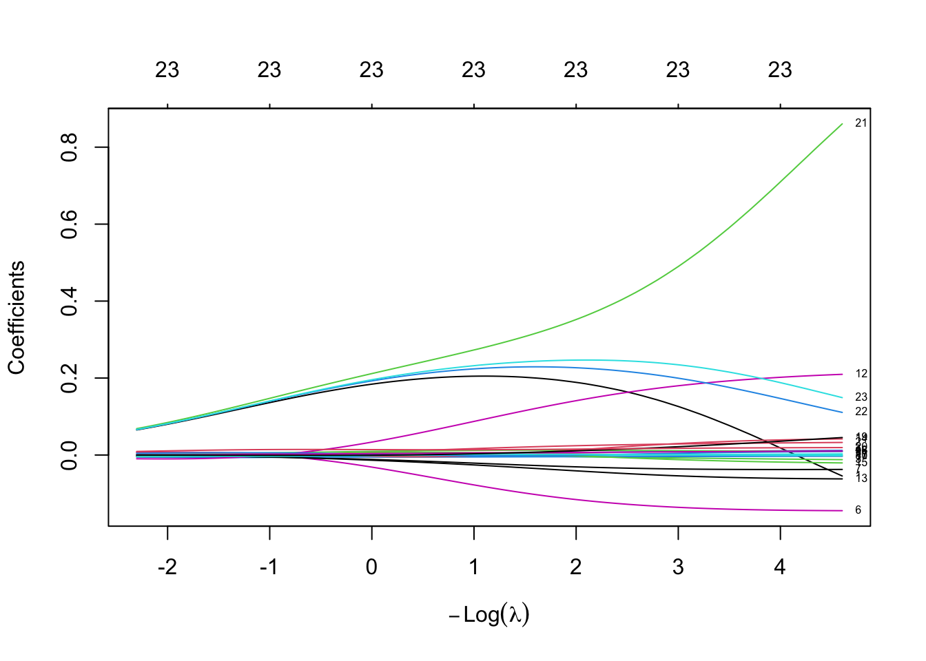
cv.ridge <- cv.glmnet(as.matrix(train.x), trainset.scaled$logprice,alpha = 0, lambda = lambda, nfolds = 10)

plot(cv.ridge)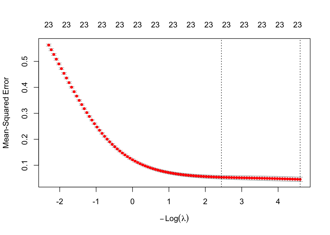
cv.ridge
Call:  cv.glmnet(x = as.matrix(train.x), y = trainset.scaled$logprice,      lambda = lambda, nfolds = 10, alpha = 0)

Measure: Mean-Squared Error

     Lambda Index Measure       SE Nonzero
min 0.01000   100 0.04562 0.008444      23
1se 0.08697    69 0.05379 0.006803      23
best_lam <- cv.ridge$lambda.min
ridge_coef <- predict(cv.ridge, s = best_lam, type = "coefficients")
ridge_coef24 x 1 sparse Matrix of class "dgCMatrix"
s=0.01
(Intercept) -1.564928e-14
carat -5.448247e-02
cut.L 3.267201e-02
cut.Q -1.197818e-02
cut.C 1.219518e-02
cut_4 2.998444e-03
color.L -1.446473e-01
color.Q -3.744780e-02
color.C -2.738590e-03
color_4 9.394073e-03
color_5 -3.019684e-03
color_6 7.682292e-04
clarity.L 2.097124e-01
clarity.Q -6.202300e-02
clarity.C 4.186375e-02
clarity_4 -2.048792e-02
clarity_5 9.100290e-03
clarity_6 -1.519407e-03
clarity_7 1.037701e-02
depth 4.537965e-02
table 1.932575e-02
x 8.605183e-01
y 1.107601e-01
z 1.491461e-01ytr.pred.ridge <- exp(predict(cv.ridge,s =best_lam, newx=as.matrix(train.x)) * sigma + mu)
yte.pred.ridge <- exp(predict(cv.ridge,s = best_lam,newx= as.matrix(test.x)) * sigma + mu)
pf.ridge <- data.frame(
model = "ridge",
train.mse = mean((ytr.pred.ridge-ytr.true)^2),
test.mse = mean((yte.pred.ridge-yte.true)^2)
)
pf.ridge model train.mse test.mse
1 ridge 391270522 2773539pf.ridge2 <- postResample(
pred = yte.pred.ridge,
obs = yte.true
)6.4.3 Elastic Net
The alpha argument of the glmnet function is described as:
\[ \frac{1-\alpha}{2} \left\|\beta \right\|_2^2 + \alpha \left\|\beta \right\|_1 \]
That’s why when we set \(\alpha = 1\) means Lasso Regression, and 0 for Ridge Regression.
6.5 Model Diagnosis
6.6 Summary
rbind(
    pf.lm,
    pf.lm.sb,
    pf.lm.sf,
    pf.lasso,
    pf.ridge
)
model train.mse test.mse
1 lm 229599179 4206268380
2 Stepwise-Backward 1200659 1243213
3 Stepwise-Forward 1200659 1243213
4 lasso 3193370 4703154
5 ridge 391270522 2773539rbind(
pf.linearRegression,
pf.Stepwise.Backward,
pf.Stepwise.Forward,
pf.lasso2,
pf.ridge2
) RMSE Rsquared MAE
pf.linearRegression 64855.751 0.01863255 2350.7410
pf.Stepwise.Backward 1114.994 0.93432609 486.5987
pf.Stepwise.Forward 1114.994 0.93432609 486.5987
pf.lasso2 2168.676 0.81577988 664.7580
pf.ridge2 1665.395 0.88162500 587.01516.7 Bad Example (Random Numbers)
x <- rnorm(50, 6,3)
y <- 10+ 2*x - 3 *x^3 -6*x^5 + 0.6 * x^7 + rnorm(50,10,8)

plot(x,y)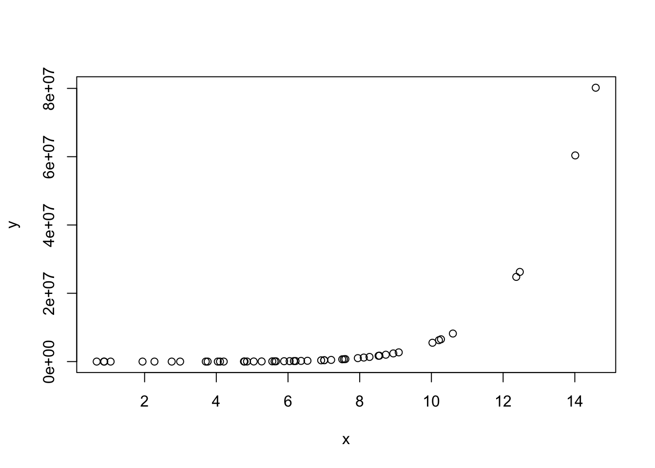
lm(y~x) %>%
    summary()
Call:
lm(formula = y ~ x)

Residuals:
     Min       1Q   Median       3Q      Max
-9551661 -7168900 -2518269  3203266 51954823

Coefficients:
             Estimate Std. Error t value Pr(>|t|)
(Intercept) -14210959    3541874  -4.012  0.00021 ***
x             2911495     486816   5.981 2.68e-07 ***
---
Signif. codes:  0 '***' 0.001 '**' 0.01 '*' 0.05 '.' 0.1 ' ' 1

Residual standard error: 11180000 on 48 degrees of freedom
Multiple R-squared:  0.427, Adjusted R-squared:  0.4151
F-statistic: 35.77 on 1 and 48 DF, p-value: 2.683e-07lm(y~x+I(x^2)+I(x^3)+I(x^4)+I(x^5)+I(x^6)+I(x^7)) %>%
summary()
Call:
lm(formula = y ~ x + I(x^2) + I(x^3) + I(x^4) + I(x^5) + I(x^6) +
    I(x^7))

Residuals:
     Min       1Q   Median       3Q      Max
-14.0609  -5.1669  -0.8895   4.8241  16.1121

Coefficients:
              Estimate Std. Error  t value Pr(>|t|)
(Intercept)  5.714e+01  2.726e+01    2.096   0.0421 *
x           -7.012e+01  5.435e+01   -1.290   0.2040
I(x^2)       4.399e+01  3.591e+01    1.225   0.2274
I(x^3)      -1.544e+01  1.123e+01   -1.376   0.1762
I(x^4)       1.855e+00  1.873e+00    0.990   0.3278
I(x^5)      -6.150e+00  1.712e-01  -35.933   <2e-16 ***
I(x^6)       6.295e-03  8.064e-03    0.781   0.4394
I(x^7)       5.999e-01  1.529e-04 3922.666   <2e-16 ***
---
Signif. codes:  0 '***' 0.001 '**' 0.01 '*' 0.05 '.' 0.1 ' ' 1

Residual standard error: 7.238 on 42 degrees of freedom
Multiple R-squared:      1, Adjusted R-squared:      1
F-statistic: 2.854e+13 on 7 and 42 DF,  p-value: < 2.2e-16