x <- seq(-20,20,0.1)
plot(x, 1/(1+exp(-x)), 'l')
title('Logistics Function')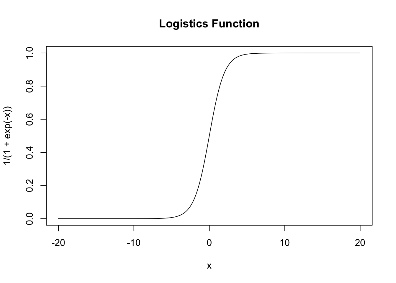
Assume you’re predicting binary categorical data with OLS:
\[ Y = \alpha + \beta X + \varepsilon \]
The problem is, \(Y \sim Bin(p)\) rather than \(N(\mu, \sigma^2)\). The target should be from \([0,1]\), indicating the probability which category this sample likely belongs to. However, the predicated value may greater than 1 or less than 0, which cause a problem.
But you can have a function to map \((-\infty, \infty)\) to \((0,1)\) which is \(y = \frac{1}{1+e^{-x}}\) (logistic function, aka. sigmoid function as activation function in neural network)
x <- seq(-20,20,0.1)
plot(x, 1/(1+exp(-x)), 'l')
title('Logistics Function')
Let \(p = \frac{1}{1+e^{-\eta}}\). Thus the model is,
\[ \eta = \log{\frac{p}{1-p}} = \alpha + \beta X + \varepsilon \]
Here we define Odds (\(\eta = \log{Odds}\)) helps explain the model.
\[ Odds = \frac{p}{1-p} \]
We use MLE to estimate, and solve by iteration. In R, we use glm function with family = binomial.
MLE function is given by
\[ L = \prod_{i = 1}^{n} {(1-p)}^{1-y_i} {p}^{y_i} = {(1-p)}^{n-\sum y_i} {p}^{\sum y_i} \]
\[ l = {(n-\sum y_i)}\log{(1-p)} + {(\sum y_i)}\log{p} \]
R utilize Iteratively Reweighted Least Squares (IRLS) to calculate the coefficients of the regression. Guess first, then iteration until likelihood function no longer increase.
For generalized model, p variables,
\[ \log{\frac{p}{1-p}} = \beta_0 + \beta_1 x_1 + \beta_2 x_2 + \dots + \beta_p x_p \]
\[ P(Y = 1) = \frac{e^{ \beta_0 + \beta_1 x_1 + \beta_2 x_2 + \dots + \beta_p x_p}}{1 + e^{ \beta_0 + \beta_1 x_1 + \beta_2 x_2 + \dots + \beta_p x_p}} \]
\[ \text{Odds Ratio} = OR = \frac{Odds_1}{Odds_2} \]
\[ \text{Relative Risk} = RR = \frac{p_1}{p_2} \rightarrow OR = RR \times \frac{1-p_1}{1-p_2} \]
Note that when p is small, \(OR \approx RR\)
to explain the model, we can write
\[ \frac{p}{1-p} = e^{\beta_0} (e^{\beta_1 })^{x_1} (e^{\beta_2 })^{x_2} \dots (e^{\beta_p })^{x_p} \]
when reply \(X\) by \(X+1\) then \[ \frac{e^{\beta_0 + \beta_1 (X+1)}}{e^{\beta_0 + \beta_1 X}} = e^{\beta_1} \]
The odds ratio \(e^{\beta} > 1\) indicates increasing odds, otherwise it’s decreasing odds.
set.seed(3306)

y <- sample(c(0,1), 20, T)
x <- y * 5 -y^2  + runif(20, 5, 10)+ rnorm(20, 5, 10)
plot(x,y)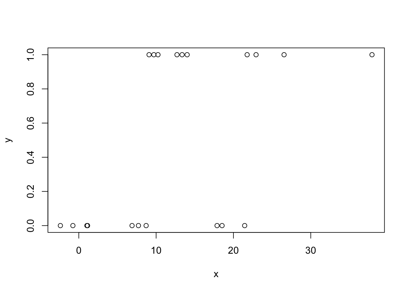
model <- glm(y ~ x, family = binomial)
summary(model)
Call:
glm(formula = y ~ x, family = binomial)

Coefficients:
            Estimate Std. Error z value Pr(>|z|)
(Intercept) -1.73353    1.00181   -1.73   0.0836 .
x            0.13851    0.07067    1.96   0.0500 *
---
Signif. codes:  0 '***' 0.001 '**' 0.01 '*' 0.05 '.' 0.1 ' ' 1

(Dispersion parameter for binomial family taken to be 1)

    Null deviance: 27.726  on 19  degrees of freedom
Residual deviance: 21.951  on 18  degrees of freedom
AIC: 25.951

Number of Fisher Scoring iterations: 4
log_or <- coef(model)["x"]
or <- exp(log_or)
list(log_or = log_or, or = or)$log_or
x
0.1385138
$or
x
1.148566 confint(model)Waiting for profiling to be done... 2.5 % 97.5 %
(Intercept) -4.08999874 -0.00682785
x 0.02215079 0.30995357For classfication models like logitics regression, Confusion Matrix is a good method to evaluate your model.
| Predicted: NO (0) (Not to Reject) |
Predicted: YES (1) (Reject Null Hypothesis) |
Total | |
|---|---|---|---|
| Actual: NO (0) (Alter is Wrong) |
True Negative (TN) | False Positive (FP) (Type I Error) |
\(N\) |
| Actual: YES (1) (Alter is Correct) |
False Negative (FN) (Type II Error) |
True Positive (TP) (Power) |
\(P\) |
| Total | \(N_{pred}\) | \(P_{pred}\) | Total (N) |
You can see there’s also a link between statistics inference and machine learning. Interesting! Note that in statistics we prefer writing \(H_0\) (Null Hypothesis) is true or false rather than then \(H_1\) (or \(H_a\), alternative hypothesis).
The first letter T or F means whether this case is correctly identified; the second letter P or N means which sample the case belongs to.
prob <- predict(model, list(x), type = "response")
predicted.classes <- ifelse(prob > 0.5, "1", "0")
table(predicted.classes,y)
y
predicted.classes 0 1
0 7 3
1 3 7From the confusion matrix, we can tell \(7+9 =16\) samples correctly classificated, and 2 of Positive and 2 of Negative mistakenly classfied into Negative and Positive respectively.
So the TP = TN = 7, FP = FN = 3.
\[\text{Accuracy} = \frac{TP+TN}{TP+TN+FP+FN}\]
\[\text{Recall} = \frac{TP}{TP+FN}\]
Recall is used to measure how many Positive Samples being correctly recognized. Assume you’re predicating whether a product has an issue, and your target is to recall samples with an issue. Recall reports in what extend you find the real issue samples.
\[\text{Specificity} = \frac{TN}{TN+FP}\]
Specificity is opposite to the Recall. The target is to find how many Negative Samples beging correctly recognized.
\[\text{Precision} = \frac{TP}{TP+FP}\]
Precision is different from either Recall and Specificity, since it measures how many samples with Positive Results really from Positive Samples. Assume you’re predicating whether a product has an issue, Precision reports whether a sample you’re recalling is really recall-needed one.
Let’s make an example. You’re doing a model about fraud detection. The higher recall indicate you find almost most fraud, while you may interupt some non-fraud transcations; the higher Precision means you’re not interupt most non-fraud transcations while may miss some fraud transcations.
F-1 Score is the Harmonic Mean of Recall and Precision
\[ \text{F-1 Score} = \frac{2}{\frac{1}{Recall}+\frac{1}{Precision}} = 2 \frac{Recall \times Precision}{Recall + Precision} \]
To avoid mistakes, use the confusion matrix function form package caret.
It’s recommand to write like caret::confusionMatrix if there’s two functions from different packages have the same name (but here we didn’t load both package, just let you know). Try to type?confusionMatrix, another function is from package ModelMetrics.
caret::confusionMatrix(
   as.factor(ifelse(prob > 0.5, "1", "0")),
   as.factor(y),
   positive = "1"
   )
Confusion Matrix and Statistics
Reference
Prediction 0 1
0 7 3
1 3 7
Accuracy : 0.7
95% CI : (0.4572, 0.8811)
No Information Rate : 0.5
P-Value [Acc > NIR] : 0.05766
Kappa : 0.4
Mcnemar's Test P-Value : 1.00000
Sensitivity : 0.70
Specificity : 0.70
Pos Pred Value : 0.70
Neg Pred Value : 0.70
Prevalence : 0.50
Detection Rate : 0.35
Detection Prevalence : 0.50
Balanced Accuracy : 0.70
'Positive' Class : 1