16 Monte Carlo
16.1 Monte Carlo Simulation of Intergation
16.1.1 Example 1
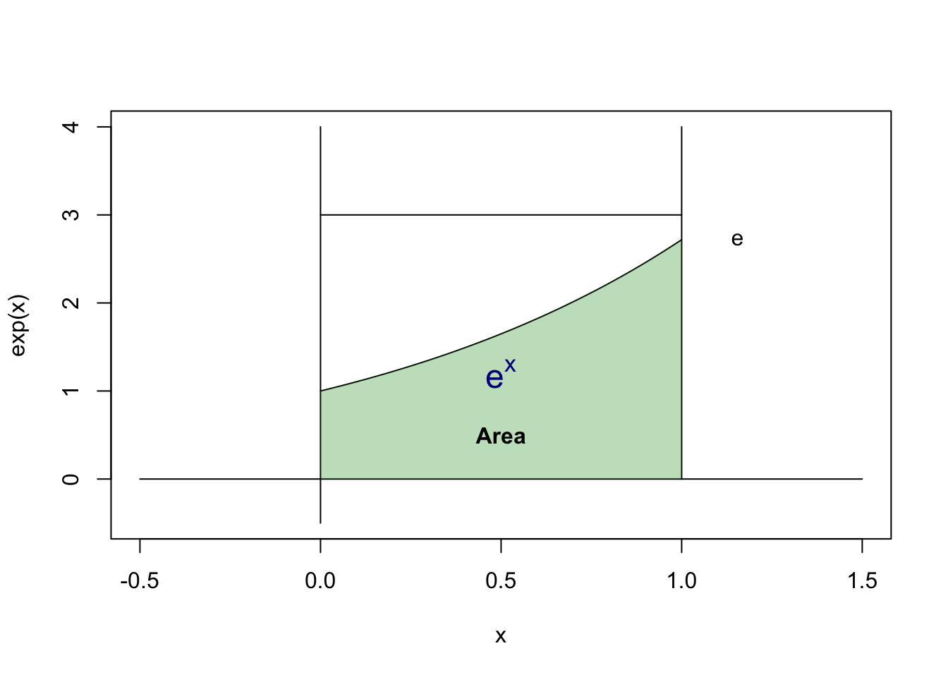
Estimating this intergal by Monte Carlo: \[ \theta = \int_{0}^{1} {e^x} dx = e-1 \]
The real integation is \(e-1\). But this is meaningless for those we can’t integrate easily.
The idea of Monte Carlo is, assuming there’s a area x from 0 to 1, y from 0 to M (a large number, greater than the maximum of function we’re estimating)
We’re calculting the green area in the plot, note that there’s a probability of random point in the green area is equal to their ratio of area.
Find any M, i.e., here we let \(M = 3 > e\)
\[ p = \frac{\text{Area of Green}}{\text{Area of Rectangular}} = \frac{S_G}{S_R} \]
Let \(X\) is a random variable with uniform distribution from 0 to 1, \(Y = e^X\), then the Intergal \(\hat{\theta} = S_G = p S_R = \mathbb{E}[\bar{Y}]\)
m <- 1000
x <- runif(m)

cat(c("Monte Carlo", mean(exp(x)), '\n'))
Monte Carlo 1.71023613681694 cat(c("Real Intergation", exp(1)-1, '\n'))Real Intergation 1.71828182845905 16.1.2 Example 2: Improper Integral
Estimating this intergal by Monte Carlo: (F(x) here is CDF of normal distribution) \[ \theta = \int_{-\infty}^{x} {\frac{1}{\sqrt{2\pi}}e^{-\frac{t^2}{2}}} dt = F(x) \]
Let’s make transformation first:
\[\theta = (0.5+ \int_{0}^{x} {\frac{1}{\sqrt{2\pi}}e^{-\frac{t^2}{2}}} dt )=\frac{1}{2}+ \frac{1}{\sqrt{2\pi}} \int_{0}^{1} xe^{-\frac{(xy)^2}{2}}dy\]
y <- runif(m)
x <- 1
cat(c("Monte Carlo", 0.5 + x / sqrt(2 * pi) * mean(exp(-(x*y)^2/2)), '\n'))
Monte Carlo 0.840837027284758 cat(c("Real Intergation", pnorm(1), '\n'))Real Intergation 0.841344746068543 Another idea is that, the sample EDF will converge to CDF. Thus, let’s generate normal random variables.
y <- rnorm(m)
x <- 1

cat(c("Monte Carlo",  mean(y<=x), '\n'))
Monte Carlo 0.842 cat(c("Real Intergation", pnorm(1), '\n'))Real Intergation 0.841344746068543 16.1.3 Variance
In the first example we use \(Y = e^X\) to estimate $ = _{0}^{1} {e^x} dx $
As \(X\sim U(0,1)\), it’s unbiased estimation since \(\mathbb{E}[Y] = \mathbb{E}[e^X] = e-1 = \theta\).
The variance is \(Var[Y] = \mathbb{E}[Y^2] - {[\mathbb{E}[Y]]}^2 = \frac{(e-1)(3-e)}{2} = 0.2420\)
[1] "variance is, 0.242035607452765"For the second example, we have two estimation:
\[X_1 \sim U(0,1) \Rightarrow Y_1 = \frac{1}{2} + \frac{1}{\sqrt{2\pi}} x e^{-\frac{xX_1}{2}}\]
x_1 <- runif(m)
x <- 1
y_1 <- 1/2+ x / sqrt(2 * pi) * exp(-(x*x_1)^2/2)
var(y_1)
[1] 0.002347814\[X_2 \sim N(0,1) \Rightarrow \frac{Y_2}{\sqrt{2\pi}}\sim B(1,p)\]
x_2 <- rnorm(m)
x <- 1
y_2 <- (x_2<=x)

var(y_2)
[1] 0.12902516.2 Variance Decrease
16.2.1 Antithetic Variates
\[U \sim U(0,1) \Rightarrow 1-U \sim U(0,1)\]
\[Z \sim N(0,1) \Rightarrow -Z \sim Z(0,1)\]
x_1 <- runif(m/2)
x <- 1
y_1a <- 1/2+ x / sqrt(2 * pi)* ((exp(-(x*x_1)^2/2) + exp(-(x*(1-x_1))^2/2))/2)
var(y_1a)
[1] 8.304542e-05var(y_1)/var(y_1a)[1] 28.27144x_2 <- rnorm(m/2)
x <- 1
y_2a <- ((x_2<=x) + (-x_2 <= x)/2)
var(y_2a)[1] 0.1374138var(y_2)/var(y_2a)[1] 0.938952316.2.2 Control Variable
Estimating \(g(U)\) with \(Var[g(U)]\), optimizing by \(h(U) = g(U) + c [f(U)-\mu]\)
Then the variance become \(Var[g[U]] + c^2 Var[f[U]] +2c COV(g(X), f(X))\), which is minimized when \(c^* = - \frac{cov(g(X), f(X))}{Var[f(U)]}\)
\[Var[h(U)] = Var[g(U)] - \frac{[COV(g(X), f(X))]^2}{[Var[f(U)]]^2} \]
Example: estimating \(\theta = \int_{0}^{1} {e^x} dx = e-1\)
m <- 1000
x <- runif(m)

y3a <- exp(x)
cat(c("Monte Carlo", mean(y3a), '\n'))
Monte Carlo 1.71288580562846 cat(c("Monte Carlo Variance", var(y3a), '\n'))Monte Carlo Variance 0.255165094190046 We use \(U \sim U(0,1)\) and \(g(U) = e^U\) as estimation. Let \(f(U) = U\) be the controling variable:
gU <- exp(x)
fU <- x
c.star = - cov(gU, fU) / var(fU)

y3b <- gU + c.star * (fU - mean(fU))

cat(c("Control Variable", mean(y3b), '\n'))
Control Variable 1.71288580562846 cat(c("Control Variable Variance", var(y3b), '\n'))Control Variable Variance 0.00395813289699567 cat(c("Variance Decrease Ratio", var(y3a)/var(y3b), '\n'))Variance Decrease Ratio 64.4660249744829 16.2.3 Importance Sampling
To estimate \(\int_{A} f(x) dx\), find another function close to \(f(x)\) on the same support, thus we have \(\int_{A} f(x) dx = \int_{A} \frac{f(x)}{g(x)} g(x) dx\)
If this the support of the distribution is equal to the A here, it will equal to the expection \(\int_{A} {f(x) dx}= \mathbb{E}{[\frac{f(x)}{g(x)}]}\)
Another format is, \(\int_{A} {f(x)g(x) dx}\) then you can give a \(h(x)\) then \(\int_{A} {f(x)g(x) dx }= \int_{A} {\frac{f(x)g(x)}{h(x)} h(x) dx}\)
16.2.3.1 Example
Let’s estimate:
\[ \omega = \int_{0}^{0.5} {e^{-x}dx} \]
Find an importance function, here we use exponential \(f(x) = \lambda e^{-\lambda x}\quad (x\geq 0 )\)
\[ \begin{array}{rl} \omega & = \int_{0}^{0.5} {e^{-x}dx} \\ & = \int_{0}^{0.5} {\frac{e^{-x}}{f(x)} f(x)dx} \\ & = \int_{0}^{0.5} {\frac{e^{-x}}{\lambda e^{-\lambda x}} \lambda e^{-\lambda x}dx} \\ & = \int_{0}^{0.5} { e^{-(1-\lambda) x} e^{-\lambda x}dx} \end{array} \]
A simple idea is to let \(\lambda = 1\), then we just calculate how many elements drop to area \([0,0.5]\). This is equalivent to the CDF of exponential, \(F(0.5)\).
set.seed(67)
omega.real <- -exp(-0.5)+1
m <- 10000
u1 <- runif(m, 0, 0.5)
omega1.est <- (0.5 - 0) * exp(-u1)

curve(dexp(x), from = 0, to = 10, xlim = c(0, 1), main = "pdf of exponential (1)")
e2 <- rexp(m)
omega2.est <- (e2 <= 0.5)

cat("real value is ", omega.real, "\n")
real value is 0.3934693 cat("general estimation is ", mean(omega1.est), "\n")general estimation is 0.3934729 cat("variance of general estimation is ", var(omega1.est), "\n")variance of general estimation is 0.003194946 cat("importance sampling estimation is ", mean(omega2.est), "\n")importance sampling estimation is 0.399 cat("variance of importance sampling estimation is ", var(omega2.est), "\n")variance of importance sampling estimation is 0.239823 The variance is very big, since we drop more than 60% of sample. A better idea is to use Beta(1,1.2) and transform into \([0,0.5]\)
curve(dexp(x), from = 0, to = 10, xlim = c(0,1), ylim = c(0,2), main = "pdf of exponential (1) and beta (1,1.2)")
curve(dbeta(x/2, 1,1.2)/2, from = 0, to = 10, xlim = c(0,1),  ylim = c(0, 2), add = T)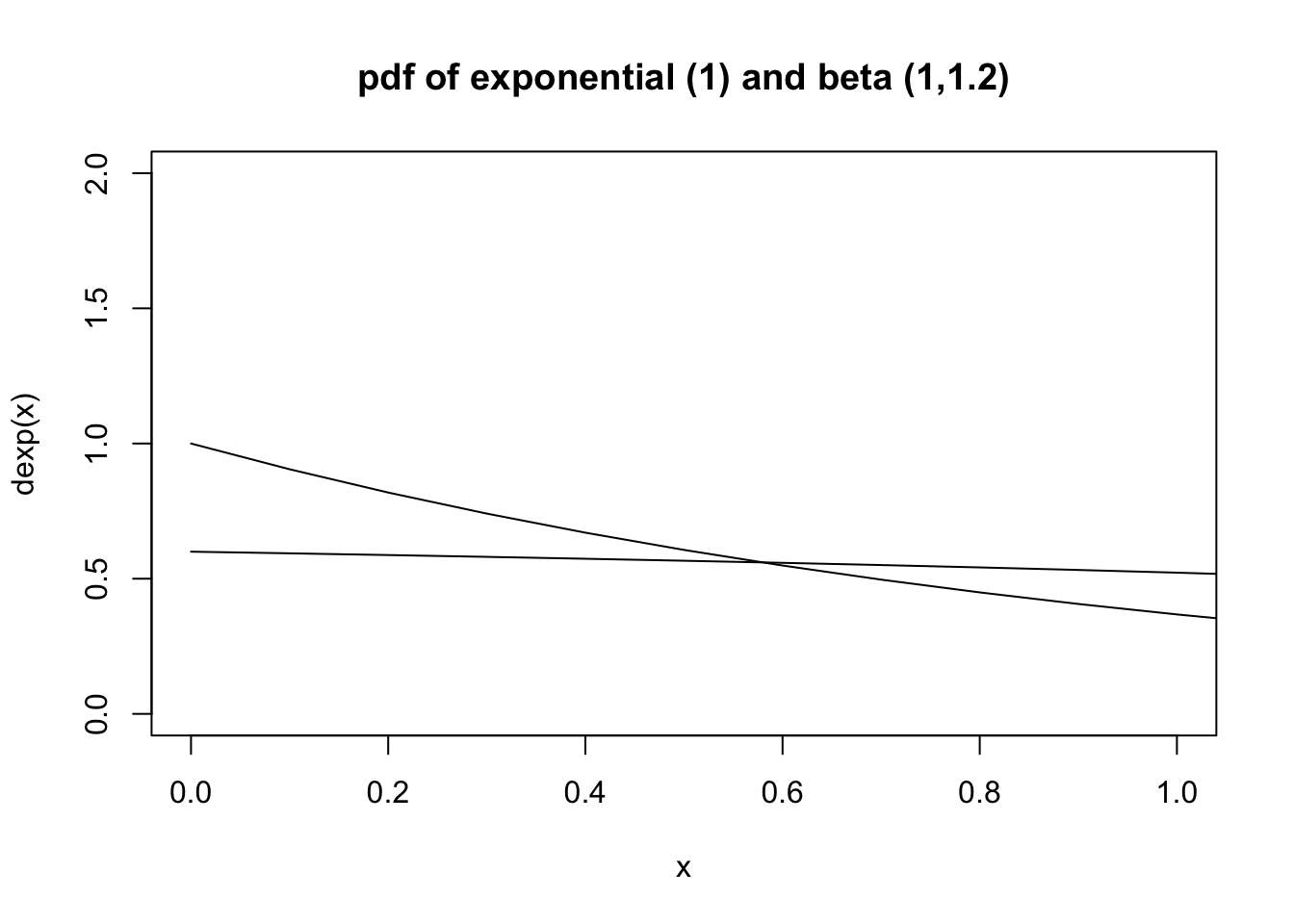
e3 <- rbeta(m,1,1.2)/2
omega3.est <- exp(-e3)/(dbeta(e3*2,1,1.2)*2)

cat("importance sampling estimation is ", mean(omega3.est), "\n")
importance sampling estimation is 0.3934025 cat("variance of importance sampling estimation is ", var(omega3.est), "\n")variance of importance sampling estimation is 0.001304244 cat("variance of general estimation is ", var(omega1.est), "\n")variance of general estimation is 0.003194946 Let’s go back to first trial: exponential trial. We use \(\lambda = 1\) is just for convenience.
lam <- 2
e2a <- rexp(m, lam)
omega2a.est <- (e2a <= 0.5) * exp((lam-1)*e2a)/lam


cat("importance sampling estimation is ", mean(omega2a.est), "\n")
importance sampling estimation is 0.3923736 cat("variance of importance sampling estimation is ", var(omega2a.est), "\n")variance of importance sampling estimation is 0.09533041 cat("variance of general estimation is ", var(omega1.est), "\n")variance of general estimation is 0.003194946