set.seed(42)15 Generate Random Variables
Reference: Rizzo (2019) Chapter 3
15.1 Remember to Set the Random Seed
If the seed is not set by a default value, each time I render the webpage, the R codes will run, and different results may given. In some documents, the text will require to change in order to match the code output. In your project, set it whatever you like, 42, 2026, 3306, 3389, 65535, 114514, …
15.2 Direct approach in R
# Uniform (0,1)
runif(n = 10, min = 0, max = 1)
[1] 0.9148060 0.9370754 0.2861395 0.8304476 0.6417455 0.5190959 0.7365883
[8] 0.1346666 0.6569923 0.7050648# Bin(30, 0.6)
rbinom(n = 10, size = 30, prob = 0.6) [1] 18 16 14 20 18 14 13 21 18 18# Poisson(7)
rpois(n = 5, lambda = 7)[1] 11 4 14 12 4# Beta(5,3)
rbeta(n = 10, shape1 = 5, shape2 = 3) [1] 0.6180147 0.3383139 0.4158620 0.4378221 0.5261561 0.4187009 0.7703246
[8] 0.5679070 0.6560498 0.552406715.3 Inverse CDF
For any continuous random variable, the random variable defined by its Cumulative Distribution Function (CDF) evaluated at itself follows a U(0,1) distribution.
Thus you can get the random value from the inverse of CDF.
15.3.1 Example: Exp(2)
\[f(x) = 2e^{-2x} \quad F(x) = 1 - e^{-2x}\]
Thus, \(U = F(x)\) we have \(x = -\frac{1}{2} \log{(1-U)}\)
- Generate \(U \sim Uniform(0,1)\) (10,000) uniform random numbers
- Compute \(X = -\frac{1}{2} \log{U}\)
m <- 100000
U <- runif(m)
X <- -1/2 * log(U)

hist(X, freq = F)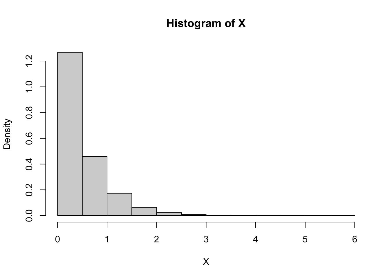
15.3.2 Example: Beta(5,3)
\[f(x) = \frac{1}{Beta(5,3)} x^4 (1-x)^2\]
ReverseCDF <- function(N) {
    return(qbeta(runif(N),5,3))
}

b0 <- ReverseCDF(50)
hist(b0, freq = F, ylim = c(0, 2.8))
curve(dbeta(x, 5, 3), add = T)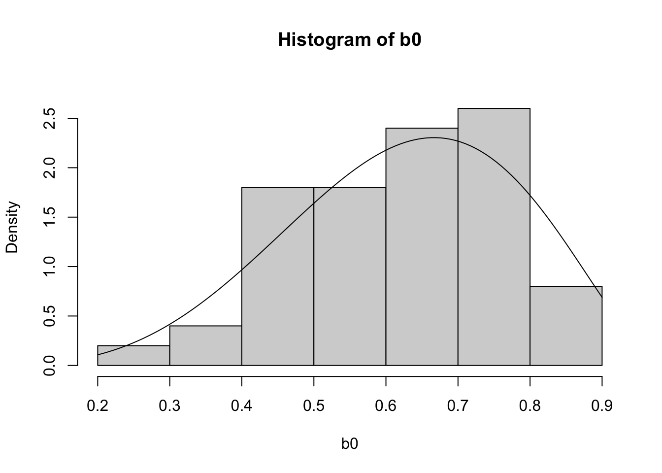
15.4 Acceptance-Rejection Method
You want to generate \(X\sim f_X\) but it’s difficult to do directly.
Assume you have \(Y\sim g_Y\) which is easy to generate, and \[ \frac{f(t)}{g(t)}\leq c, \forall t \text{ s.t. } f(t)>0 \]
Then generate \(u\) from \(U \sim U(0,1)\) and \(y\) from \(Y\sim g_Y\), accept \(y\) if \(u < \frac{f(t)}{c g(t)}\), otherwise drop it.
In some textbooks, \(M = sup \frac{f(t)}{g(t)} < \infty \Rightarrow \frac{f(t)}{Mg(t)}\leq 1\). The \(M\) here is equal to the \(c\) mentioned earlier.
15.4.1 Example: Beta(5,3)
\[f(x) = \frac{1}{Beta(5,3)} x^4 (1-x)^2\]
\[f'(x) = \frac{1}{Beta(5,3)} [4x^3 (1-x)^2 - 2x^4 (1-x)] = \frac{2x^3(1-x)(2-3x)}{Beta(5,3)} \]
Then we have \(M = sup \frac{f(t)}{g(t)} = f(\frac{2}{3})\)
b1 <- rbeta(50, 5,3)
hist(b1, freq = F, ylim = c(0, 2.8))
curve(dbeta(x, 5, 3), add = T)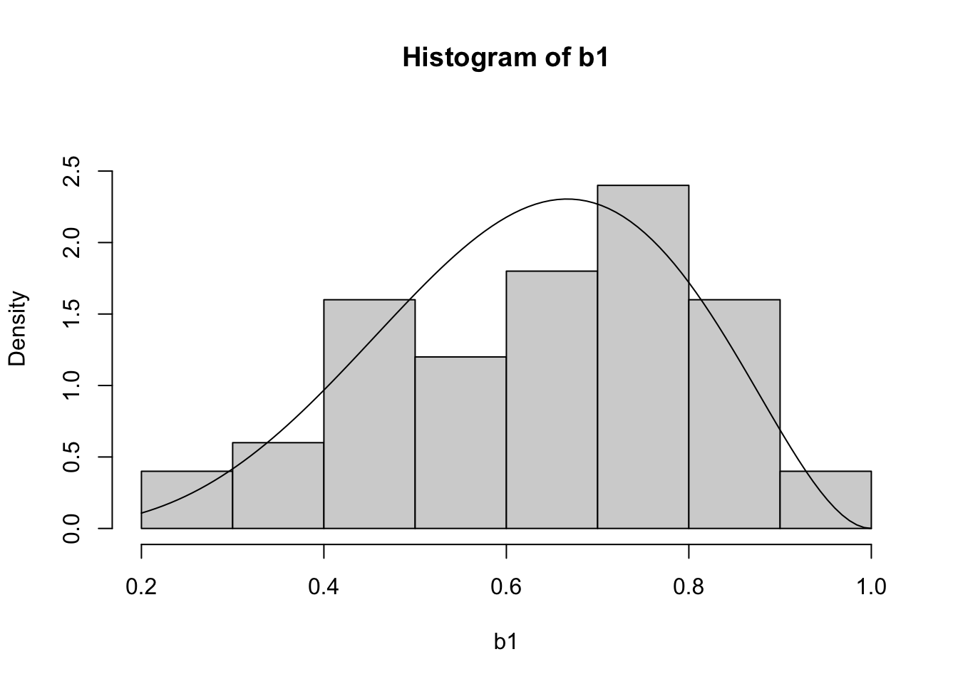
b2 <- c()
M <- dbeta(2/3, 5,3)
while (length(b2) < 50){
    u1 <- runif(1)
    y <- runif(1)
    if(u1 < dbeta(y,5,3)/M){
        b2 <- c(b2,y)
    }
}
hist(b2, freq = F, ylim = c(0, 2.8))
curve(dbeta(x, 5, 3), add = T)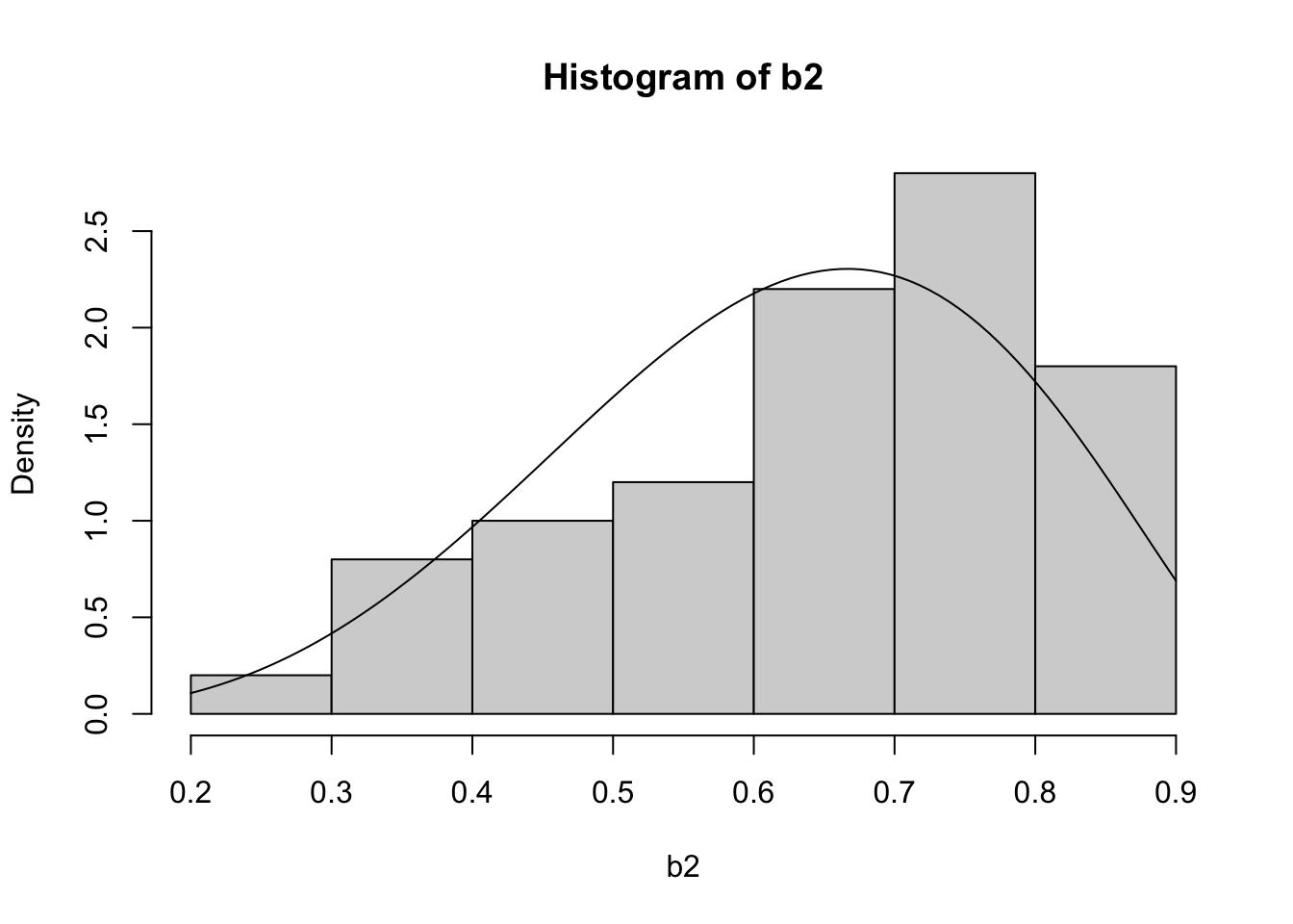
There’re some performance weakness: - bad append operation b2 <- c(b2,y) - non-vectorized operation
Let’s optimize!
N <- 50
M <- dbeta(2/3, 5,3)
N1 <- as.integer(N * M * 1.2)

u <- runif(N1)
y <- runif(N1)
b3 <- y[u < dbeta(y,5,3)/M]
print(paste(c("target is", N, ", and we generated", N1, "finally get", length(b3)), collapse = " "))
[1] "target is 50 , and we generated 138 finally get 54"b3 <- b3[1:N]
hist(b3, freq = F, ylim = c(0, 2.8))
curve(dbeta(x, 5, 3), add = T)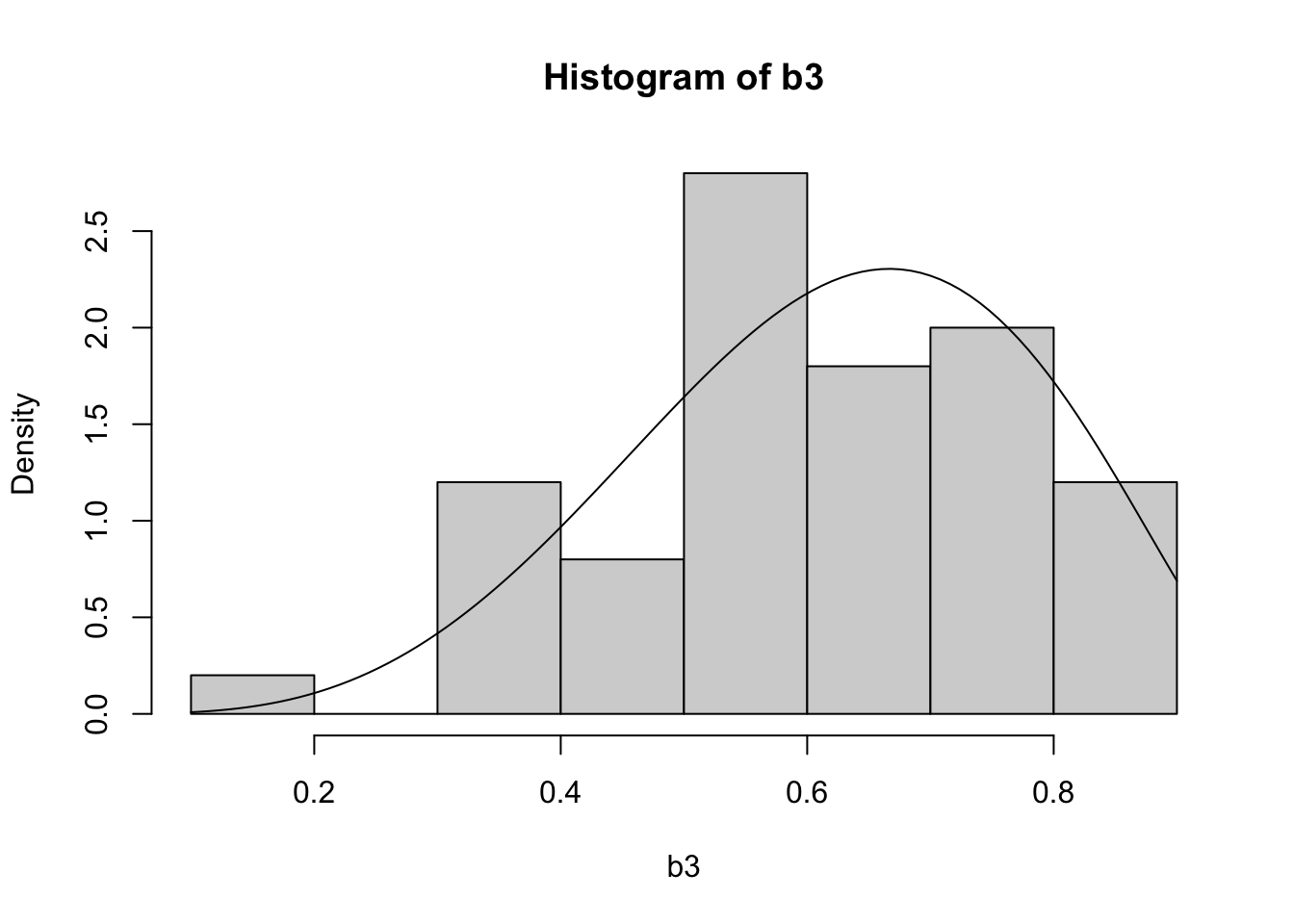
15.4.2 Example: Beta(2,2)
M <- dbeta(0.5,2,2)
mb <- as.integer(m/M * 1.2)
U <- runif(mb)
Y <- runif(mb)

X <- Y[U < dbeta(Y,2,2)/M]

hist(X, freq=F)
curve(dbeta(x,2,2), add = T)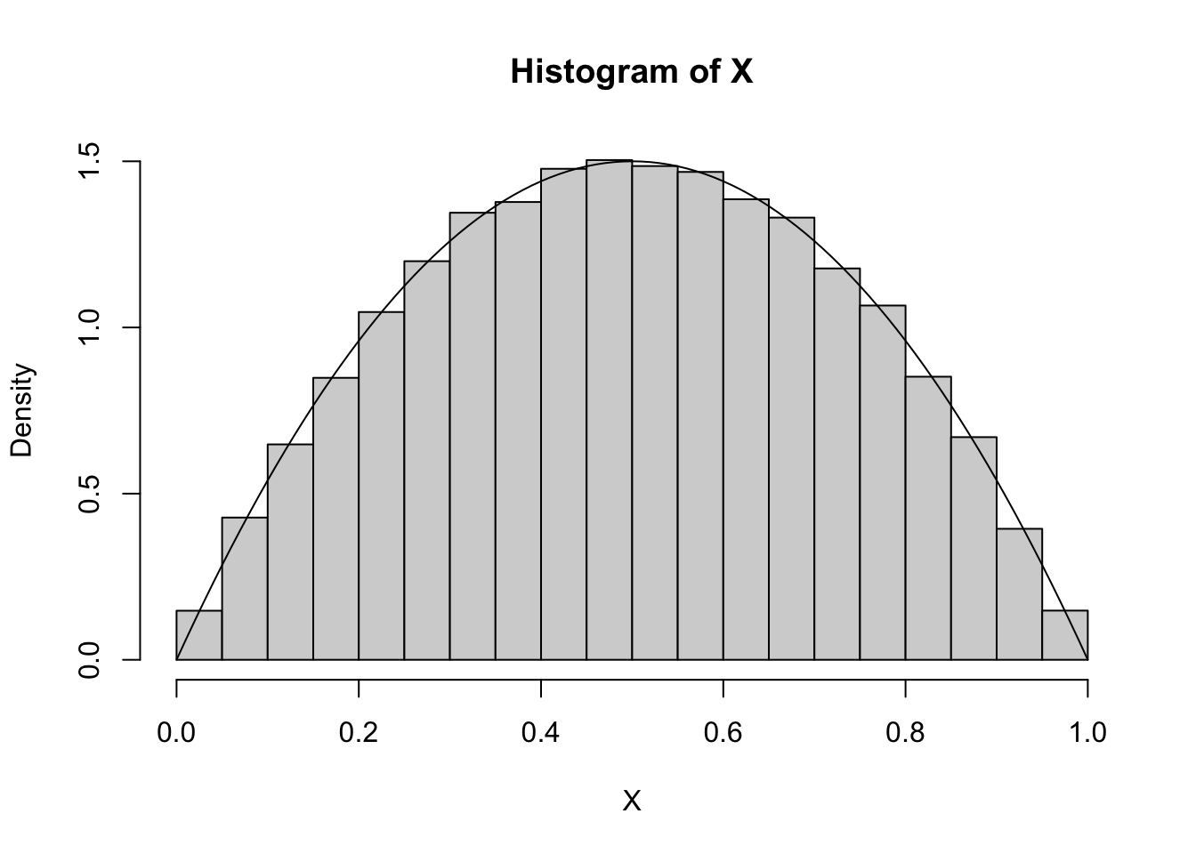
15.5 Transformation Method
iid series \(X_i \sim \Gamma(\alpha_i,\lambda) \\ \implies \frac{\sum_{k=1}^{i}X_k}{\sum_{k=1}^{i+1}X_k}\sim Beta(\sum_{k=1}^{i}\alpha_k,\alpha_{i+1})\) and \(\sum_{k=1}^{n}X_k \sim \Gamma(\sum_{i=1}^{n} \alpha_i,\lambda)\) independent
\[ U,V \stackrel{iid}{\sim} U(0,1) \to \left\{ \begin{array}{cl} Z_1 & = \sqrt{-2\log U}cos{2\pi V} \\ Z_2 & = \sqrt{-2\log V}cos{2\pi U} \end{array}\right., Z_1, Z_2 \stackrel{iid}{\sim} N(0,1) \]
m <- 100000
U1 <- runif(m)
U2 <- runif(m)
X1 <- sqrt(-2*log(U1)) * cos(2 * pi * U2)
X2 <- sqrt(-2*log(U1)) * sin(2 * pi * U2)

cor(X1, X2)
[1] 0.00217154par(mfrow = c(1,2))
hist(X1)
hist(X2)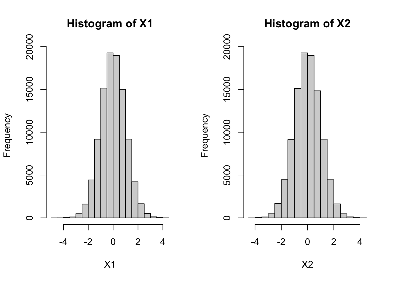
par(mfrow = c(1, 1))15.6 Benchmark
library(microbenchmark)

rejection_scalar <- function(N) {
    b2 <- numeric(N)
    M <- dbeta(2/3, 5, 3)
    count <- 0
    while (count < N) {
        u1 <- runif(1)
        y <- runif(1)
        if (u1 < dbeta(y, 5, 3) / M) {
            count <- count + 1
            b2[count] <- y
        }
    }
    return(b2)
}

rejection_vectorized <- function(N) {
    M <- dbeta(2/3, 5,3)
    N1 <- as.integer(N * M * 1.2)

    u <- runif(N1)
    y <- runif(N1)
    b3 <- y[u < dbeta(y,5,3)/M]
    return(b3[1:N])
}

results <- microbenchmark(
    Reverse = ReverseCDF(5000),
    Scalar_Loop = rejection_scalar(5000),
    Vectorized  = rejection_vectorized(5000),
    Built_in = rbeta(5000, 5, 3),
    times = 100
)
Warning in microbenchmark(Reverse = ReverseCDF(5000), Scalar_Loop =
rejection_scalar(5000), : less accurate nanosecond times to avoid potential
integer overflowsresultsUnit: microseconds
expr min lq mean median uq max
Reverse 1998.422 2037.475 2162.1112 2046.1870 2058.7945 8636.363
Scalar_Loop 11364.011 11982.496 12373.5610 12291.5335 12674.6580 14935.890
Vectorized 706.430 716.229 771.9250 722.5225 733.8385 3665.482
Built_in 246.943 250.756 255.2385 252.8675 256.3115 305.655
neval cld
100 a
100 b
100 c
100 dChi-Square
m = 1000
u1 <- rnorm(m, 0, 1)
u2 <- rnorm(m, 0, 1)
u3 <- rnorm(m, 0, 1)

csq.df3 <- u1^2+u2^2+u3^2

hist(csq.df3, breaks = 30, probability = TRUE, col = "lightblue",
     main = "Histogram of 1,000 Chi-Squared Random Variables (df = 3)",
     xlab = "Value", ylab = "Density")

curve(dchisq(x, df = 3), add = TRUE, col = "red", lwd = 2)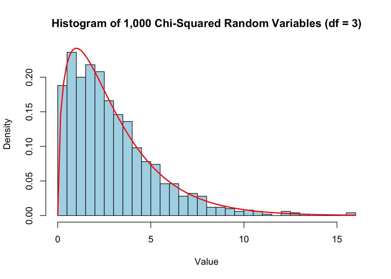
m  <- 1000
weights <- c(0.2, 0.5, 0.3)
Y <- sample(1:3, size = m, replace = T, prob = weights)
X <- numeric(m)

for(i in 1:m){
    if(Y[i] == 1){
        X[i] = rnorm(1)
    }else if(Y[i] == 2){
        X[i] = rnorm(1,-1,1)
    }else{
        X[i] = rnorm(1,2,1)
    }
}

hist(X, freq = F)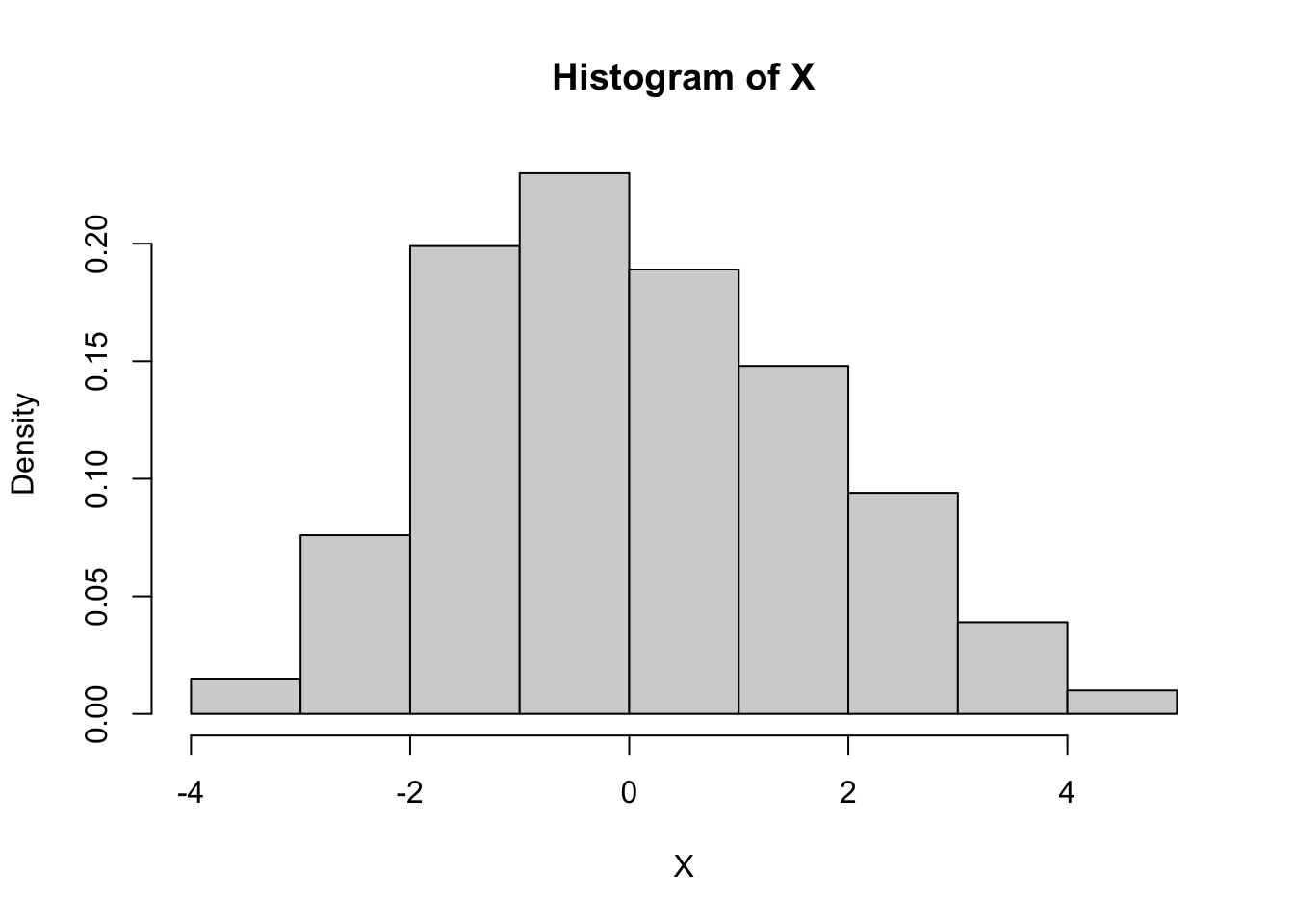
hist(X, breaks = 30, probability = TRUE, col = "lightblue",
    #  main = "Histogram of 1,000 Chi-Squared Random Variables (df = 3)",
     xlab = "Value", ylab = "Density")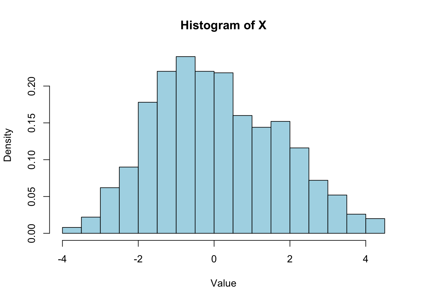
X2 <- numeric(m)

mu <- c(0,-1,2)
for (j in 1:3){
    X2[Y==j] = rnorm(sum(Y==j), mu[j])
}
hist(X2, freq = F)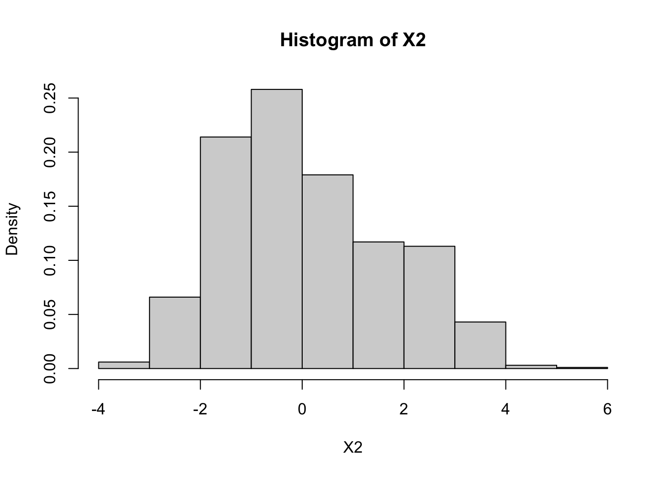
hist(X2, breaks = 30, probability = TRUE, col = "lightblue",
    #  main = "Histogram of 1,000 Chi-Squared Random Variables (df = 3)",
     xlab = "Value", ylab = "Density")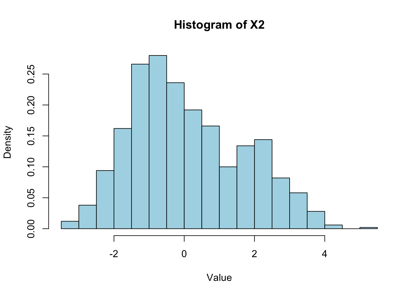
15.7 Multivariate Normal
Generate \(N_p(\mu, \Sigma)\)
with example \(\mu = \begin{bmatrix} 0 \\ 0 \\ 0 \end{bmatrix}\) and \(\Sigma = \begin{bmatrix} 2 & 1 & 1 \\ 1 & 2 & 1 \\ 1 & 1 & 2 \end{bmatrix}\)
\(\Sigma = Q^T Q\) where
We can use eigen decomposition
Here we can also use Cholesky Factorization \(A = L L*\) and L is a lower triangular matrix (in R, chol() returns utm),
\[X = ZQ + J \mu^T\]
\[Var(X) = Var(ZQ + J \mu^T) = Var(ZQ) = Q^T Var(Z) Q = Q^T Q = \Sigma\]
m <- 10000
p <- 3
mu <- matrix(c(0,0,0))
variance <- matrix(c(2,1,1,1,2,1,1,1,2), 3,3)

Z <- matrix(rnorm(m * p), m,p)
Q <- chol(variance)


X <- Z %*% Q + matrix(rep(1,m)) %*% t(mu)
# X

apply(X, 2, mean)
[1] 0.034510166 0.009282841 0.004482722cor(X) [,1] [,2] [,3]
[1,] 1.0000000 0.4873324 0.4917051
[2,] 0.4873324 1.0000000 0.4963650
[3,] 0.4917051 0.4963650 1.0000000